
Perpetual student. Interested in Maths, Computer Science and Machine Learning.
Within the field of statistics there are two prominent schools of thought, with opposing views: the Bayesian and the Classical (also called Frequentist). Their fundamental difference relates to the nature of the unknown models or variables. In the Bayesian view, they are treated as random variables with known distributions. In the classical view, they are treated as deterministic quantities that happen to be unknown.
Most classical inference problems can be identified as being one of three types: point estimation, interval estimation, or hypothesis testing. We covered point estimation and interval estimation in the previous article; here we will go over hypothesis testing.
As discussed previous, let us suppose that we observe a random sample from a population distribution, specified except for a vector of unknown parameters. However, rather than wishing to explicitly estimate the unknown parameters, let us now suppose that we are primarily concerned with using the resulting sample to test some particular hypothesis concerning them. A statistical hypothesis is usually a statement about a set of parameters of a population distribution. It is called a hypothesis because it is not known whether or not it is true. A primary problem is to develop a procedure for determining whether or not the values of a random sample from this population are consistent with the hypothesis. We start with some default theory - called a null hypothesis - and we ask if the data provides sufficient evidence to reject the theory. If not, we retain/accept the null hypothesis. Note that in accepting a given hypothesis we are not actually claiming that it is true but rather we are saying that the resulting data appear to be consistent with it.
Coin Tossing Example: Let
\[X_1, \dots, X_n \sim \mathrm{Bernoulli}(p)\]be $n$ independent coin flips. Suppose we want to test if the coin is fair. Let $H_0$ denote the hypothesis that the coin is fair and let $H_1$ denote the hypothesis that the coin is not fair. $H_0$ is called the null hypothesis and $H_1$ is called the alternative hypothesis. We can write the hypotheses as
\[H_0 : p = 1/2 \textrm{ versus } H_1: p \neq 1/2\]It seems reasonable to reject $H_0$, if $T= \vert \hat{p}_ n - \frac{1}{2} \vert$ is large.
Consider a population having distribution $F_θ$ , where $θ$ is unknown, and suppose we want to test a specific hypothesis about $θ$. We shall denote this hypothesis by $H_0$ (null hypothesis). Note: A hypothesis that, when true, completely specifies the population distribution is called a simple hypothesis; one that does not is called a composite hypothesis.
Suppose now that in order to test a specific null hypothesis $H_0$, a population sample of size $n$ — say $X_1,\dots,X_n$ — is to be observed. Based on these $n$ values, we must decide whether or not to accept $H_0$. A test for $H_0$ can be specified by defining a region $C$ in $n$-dimensional space with the proviso that the hypothesis is to be rejected if the random sample $X_1, \dots , X_n$ turns out to lie in $C$ and accepted otherwise. The region $C$ is called the critical region. In other words, the statistical test determined by the critical region $C$ is the one that rejects $H_0$ if $(X_1, \dots, X_n) \in C$ and accepts $H_0$ if $(X_1, \dots, X_n) \notin C$.
It is important to note when developing a procedure for testing a given null hypothesis $H_0$ that, in any test, two different types of errors can result. The first of these, called a type I error, is said to result if the test incorrectly calls for rejecting $H_0$ when it is indeed correct. The second, called a type II error, results if the test calls for accepting $H_0$ when it is false.
To keep type I error low, $H_0$ should only be rejected if the data is very unlikely when $H_0$ is true. The classical way of accomplishing this is to specify a value $\alpha$ and then require the test to have the property that whenever $H_0$ is true its probability of being rejected is never greater than $\alpha$. The value $\alpha$ is called the level of significance of the test. Basically Significance Level is the probability of getting a Type I error (probability of false rejection).
The $p$-value, or the probability value, is the probability of seeing a result as extreme or more extreme than yours - assuming that the null hypothesis ($H_0$) is true. If the $p$-value is low, it means the probability of that outcome under $H_0$ is low (high surprise value). If $p$-value is high, it means the observation is relatively common under the null hypothesis. $H_0$ is accepted if the significance level $\alpha$ is less than the $p$-value and rejected if it is greater than or equal.
How do we come up with a test of significance level $\alpha$? Suppose we are interested in testing a certain hypothesis concerning $\theta$, an unknown parameter of the population. Specifically, for a given set of parameter values $w$, suppose we are interested in testing
\[H_0 : \theta \in w\]A common approach to developing a test of $H_0$, say at level of significance $\alpha$, is to start by determining a point estimator of $θ$ — say $d(X)$. The hypothesis is then rejected if $d(X)$ is “far away” from the region $w$. However, to determine how “far away” it need be to justify rejection of $H_0$, we need to determine the probability distribution $d(X)$ when $H_0$ is true since this will usually enable us to determine the appropriate critical region so as to make the test have the required significance level $\alpha$.
Suppose that $X_1, . . . , X_n$ is a sample of size $n$ from a normal distribution having an unknown mean $\mu$ and a known variance $\sigma^2$ and suppose we are interested in testing the null hypothesis $H_0: \mu = \mu_0$ against the alternative hypothesis $H_1: \mu \neq \mu_0$.
Since $\bar{X} = \sum_i \frac{X_i}{n}$ is a natural point estimator of $\mu$, it seems reasonable to accept $H_0$ if $X$ is not too far from $\mu_0$. That is, the critical region of the test would be of the form
\[C = \{X_1, \dots, X_n : \;\vert\bar{X} - \mu_0\vert > c\}\]for some suitably chosen value $c$. If we desire that the test has significance level $\alpha$, then we must determine the critical value $c$ that will make the type I error equal to $\alpha$. That is, $c$ must be such that
\[\prob_{\mu_0}(\vert\bar{X} - \mu_0\vert > c) = \alpha\]where we write $\prob_{\mu_0}$ to mean that the preceding probability is to be computed under the assumption that $\mu = \mu_0$. However, when $\mu=\mu_0$, $\bar{X}$ will be normally distributed with mean $\mu_0$ and variance $\sigma^2/2$ and so $Z$, defined by
\[Z \equiv \frac{\bar{X} - \mu_0}{\sigma/\sqrt{n}}\]will have a standard normal distribution. Therefore, we have
\[\begin{align} \prob \bigg\{ \vert Z \vert > \frac{c\sqrt{n}}{\sigma} \bigg\} &= \alpha \\ \implies \prob \bigg\{ Z > \frac{c\sqrt{n}}{\sigma} \bigg\} &= \alpha/2 \\ \end{align}\]We know that
\[P(Z > z_{\alpha/2}) = \alpha/2\]Therefore,
\[\begin{align} \frac{c\sqrt{n}}{\sigma} &= z_{\alpha/2} \\ \implies c &= \frac{(\sigma) (z_{\alpha/2})}{\sqrt{n}} \end{align}\]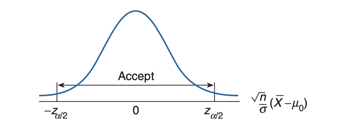
In the example above, our test statistic is $S = \frac{\bar{X} - \mu_0}{\sigma/\sqrt{n}}$. The $p$-value of this statistic is $\prob(\vert Z \vert > \vert S \vert )$.
One-sided Test
What happens when we reject the null hypothesis ($\mu = \mu_0$) only when $\mu$ is greater than $\mu_0$? That is, what happens when the alternative hypothesis to $H_0: \mu = \mu_0$ is $H_1 : \mu > \mu_0$? Clearly, in this case we would not want to reject $H_0$ when $\bar{X}$ is small (since a small $\bar{X}$ is more likely when $H_0$ is true than when $H_1$ is true). Thus, we should reject $H_0$ when $\bar{X}$, the point estimate of $\mu$, is much greater than $\mu_0$. That is, the critical region should be of the following form:
\[C = \big\{(X_1, \dots, X_n): \bar{X} - \mu_0 > c \big\}\]Since the probability of rejection should equal $\alpha$ when $H_0$ is true
\[\begin{align} &\prob_{\mu_0}\bigg\{ \bar{X} - \mu_0 > c \bigg\} = \alpha \\ \implies &\prob(Z > \frac{c\sqrt{n}}{\sigma}) = \alpha \\ \implies &\frac{c\sqrt{n}}{\sigma} = z_{\alpha} & \text{as } \prob(Z > z_\alpha) = \alpha \\ \implies & c = \frac{z_\alpha \sigma}{\sqrt{n}} \end{align}\]To compute the $p$-value in the one-sided test, we first use the data to determine the value of the statistic. The $p$-value is then equal to the probability that a standard normal would be at least as large as this value.
Up to now we have supposed that the only unknown parameter of the normal population distribution is its mean. However, the more common situation is one where the mean $\mu$ and variance $\sigma^2$ are both unknown. Consider a test of $H_0: \mu = \mu_0$ versus the alternative $H_1: \mu \neq \mu_0$. It should be noted that the null hypothesis is not a simple hypothesis since it does not specify the value of $\sigma^2$.
As before, it seems reasonable to reject $H_0$ when the sample mean $X$ is far from $\mu_0$. However, how far away it need be to justify rejection will depend on the variance $\sigma^2$. Now when $\sigma^2$ is no longer known, it seems reasonable to estimate it by
\[S^2 = \frac{\sum_i(X_i - \bar{X})^2}{n-1}\]and then to reject $H_0$ when
\[\left\vert \frac{\bar{X} - \mu_0}{S/\sqrt{n}} \right\vert\]is large. To determine how large the statistic needs to be for rejection, in order that the resulting test have significance level $\alpha$, we must determine the probability distribution of this statistic when $H_0$ is true. We know that the statistic $T$, defined by
\[T = \frac{\bar{X} - \mu_0}{S/\sqrt{n}}\]follows a t-distribution with $n-1$ degrees of freedom. Hence,
\[\prob_{\mu_0}\bigg\{ \left\vert \frac{\bar{X} - \mu_0}{S/\sqrt{n}} \right\vert \geq t_{\alpha/2, n-1} = \alpha \bigg\}\]If we let $t$ denote the observed value of the test statistic $T$ (defined above), then the $p$-value of the test is the probability that $\vert T \vert$ would exceed $ \vert t \vert$ when $H_0$ is true. That is, the $p$-value is the probability that the absolute value of a $t$-random variable with $n − 1$ degrees of freedom would exceed $ \vert t\vert$. The test then calls for rejection at all significance levels higher than the $p$-value and acceptance at all lower significance levels.
Suppose that $X_1, \dots , X_n$ and $Y_1, \dots, Y_m$ are independent samples from normal populations having unknown means $\mu_x$ and $\mu_y$ but known variances $\sigma_x^2$ and $\sigma_y^2$. Let us consider the problem of testing the hypothesis
\[H_0: \mu_x = \mu_y \text{ versus } H_1 : \mu_x \neq \mu_y\]Since $\bar X$ is an estimate of $\mu_x$ and $\bar Y$ of $\mu_y$, it follows that $\bar X − \bar Y$ can be used to estimate $\mu_x − \mu_y$. Hence, because the null hypothesis can be written as $H_0 : \mu_x − \mu_y = 0$, it seems reasonable to reject it when $\bar{X} − \bar{Y}$ is far from zero. That is, the form of the test should be to reject $H_0$ if $\vert \bar{X} − \bar{Y} \vert > c$ and accept $H_0$ otherwise, or some suitably chosen value $c$.
To determine that value of c that would result in the test having a significance level $\alpha$, we need determine the distribution of $\bar{X} − \bar{Y}$ when $H_0$ is true. From [Section 7.3.2, Confidence Intervals for the Variance of a Normal Distributions] of the book [Introduction to Probability and Statistics, Sheldon Ross], we know that
\[\bar{X} − \bar{Y} \sim \mathcal{N}(\mu_x - \mu_y, \frac{\sigma_x^2}{n} + \frac{\sigma_y^2}{m})\]which implies that
\[\frac{\bar{X} − \bar{Y} - (\mu_x - \mu_y)}{\sqrt{\frac{\sigma_x^2}{n} + \frac{\sigma_y^2}{m}}} \sim \mathcal{N}(0, 1)\]Hence, when $H_0$ is true (and so $\mu_y − \mu_y = 0$), it follows that
\[\frac{\bar{X} − \bar{Y} }{\sqrt{\frac{\sigma_x^2}{n} + \frac{\sigma_y^2}{m}}} \sim \mathcal{N}(0, 1)\]We want
\[\prob_{\mu_x = \mu_y}\bigg\{ \frac{\bar{X} − \bar{Y} }{\sqrt{\frac{\sigma_x^2}{n} + \frac{\sigma_y^2}{m}}} \notin C \bigg\} = 1 - \alpha\]Also,
\[\prob_{\mu_x = \mu_y}\bigg\{ -z_{\alpha/2} \leq\frac{\bar{X} − \bar{Y} }{\sqrt{\frac{\sigma_x^2}{n} + \frac{\sigma_y^2}{m}}} \leq z_{\alpha/2} \bigg\} = 1 - \alpha\]Therefore, the acceptance region is
\[\frac{\vert\bar{X} − \bar{Y}\vert}{\sqrt{\frac{\sigma_x^2}{n} + \frac{\sigma_y^2}{m}}} \leq z_{\alpha/2}\]