
Perpetual student. Interested in Maths, Computer Science and Machine Learning.
Within the field of statistics there are two prominent schools of thought, with opposing views: the Bayesian and the Classical (also called Frequentist). Their fundamental difference relates to the nature of the unknown models or variables. In the Bayesian view, they are treated as random variables with known distributions. In the classical view, they are treated as deterministic quantities that happen to be unknown.
Most classical inference problems can be identified as being one of three types: point estimation, interval estimation, or hypothesis testing. Here we will discuss point estimation and interval estimation, and cover hypothesis testing in the next article.
Point Estimation refers to providing a single “best guess” of some quantity of interest. The quantity of interest could be a parameter in parametric model, a CDF $F$, a probability density function $f$ or a regression function $r$.
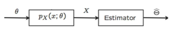
The observation $X = (X_1, \dots, X_n)$ is a random variable, whose probability distribution depends on the value of $\theta$. This probability distribution is denoted by $p_X(x;\theta)$. Remember that this indicates that $p_X$ is dependent on $\theta$, not that it is conditioned on $\theta$ in the probablistic sense.
Our task is to come up with an estimate $\hat{\Theta}$. The estimate is decided on the basis of the observations $X$ made during the experiment; $\hat{\Theta} = g(X)$. Recall that a function of a random variable is a random variable itself. Thus, $\hat{\Theta}$ is also a random variable. Each time we conduct the experiment, $X$ takes the value $x$ and $\hat{\Theta}$ takes a value $\hat{\theta}$. The set of all possible values of $\hat{\Theta}$ is called the model and $g$ is called the estimator function. The estimator function should be such that it gives a close enough estimate of $\theta$ for all possible values of $\theta$.
Sometimes, particularly when we are interested in the role of the number of observations $n$, we use the notation $\hat\Theta_n$ for an estimator. The distribution of $\hat\Theta_n$ is called the sampling distribution and is generally dependent on $\theta$. The mean and variance of $\hat\Theta_n$ are denoted by $\expect_\theta[\hat\Theta_n]$ and $\v_\theta[\hat\Theta_n]$ respectively, and the expectation is taken over all $X$ ($n$-datasets). Both $\expect_\theta[\hat\Theta_n]$ and $\v_\theta[\hat\Theta_n]$ are numerical functions of $\theta$, but for simplicity, when the context is clear we sometimes do not show this dependence.
The following are some of the desirable properties that we look for, from an estimator:
The estimation error denoted by $\tilde\Theta_n$ is defined by $\tilde\Theta_ n = \hat\Theta_n - \theta$. The bias of the estimator, denoted by $\mathrm{b}_ \theta(\hat\Theta_ n)$ is the expected value of the estimation error:
\[\mathrm{b}_\theta(\hat\Theta_n) = \expect_\theta[\hat\Theta_n] - \theta\]The estimation error depends on every observation, but the bias only depends on $\theta$ . If the bias is zero, for every possible value of $\theta$ , then we have an unbiased estimator, and this is a desirable property.
We call an estimator consistent if the sequence $\hat\Theta_n$ converges to the true value of the parameter $\theta$, in probability, for every possible value of $\theta$.
\[\hat\Theta_n \xrightarrow{n \to \theta} \theta\]Besides the bias, we are usually interested in the size of the estimation error. This is captured by the mean squared error $\expect_\theta[\tilde\Theta_n^2]$.
\[\begin{align} \expect_\theta[\tilde{\Theta}_n^2] &= \expect[(\hat\Theta - \theta)^2] \\ &= \v(\hat\Theta - \theta) + (\expect[\hat\Theta - \theta])^2 \\ &= \v(\hat\Theta) + (\expect[\hat\Theta] - \theta)^2 \\ &= \v_\theta(\hat\Theta) + \mathrm{b}^2_\theta(\hat\Theta_n) \\ \end{align}\]This formula is important because in many statistical problems, there is a trade-off between the two terms on the right-hand-side. Often a reduction in the variance is accompanied by an increase in the bias. In case of an unbiased estimator $\expect_\theta[\tilde\Theta_n^2] = \v_\theta(\hat\Theta_n)$. If we take a dumb estimator which always gives out an estimate of $0$, irrespective of the observation, then
\[\expect_\theta[\tilde\Theta_n^2] = \v(\hat\Theta_n) + \textrm{bias} = 0 + (0 - \theta)^2 = \theta^2\]Of course, a good estimator is the one that manages to keep both terms small.
Example (Expected Value Estimation) Let $X_1, \dots, X_n \sim$ Bernoulli($p$). We want to estimate the expected value of our distribution, namely $p$. Let our estimator be
\[\hat p_n = \frac{1}{n}\sum_i{X_i}\]Then, $\expect[\hat p_n] = \frac{1}{n}\sum_i \expect(X_i) = p$. Therefore, $\hat p_n$ is unbiased. The variance is $\v(\hat p_n) = \frac{p(1-p)}{n}$. As $p$ is unknown, the standard deviation of $\hat p_n$ is also unknown. This quantity is generally referred to as the standard error.
\[\text{standard error} = \sqrt{\v{(\hat\Theta_n)}}\]The estimated standard error is denoted by $\hat{\mathrm{se}}$. For our example, the estimated standard error is $\hat{\mathrm{se}} = \sqrt{\frac{\hat{p}(1-\hat{p})}{n}}$
Example (Maximum Likelihood Estimation) We have seen that if the unknown parameter can be expressed in the form of expected value of $X$, then $\hat{\Theta}$ can be taken to be the sample mean. But what if there is no apparent way of treating $\theta$ as an expectation of $X$? In that case, we will use the approach of Maximum Likelihood Estimation. We will pick $\theta$ that makes the data most likely.
\[\hat\theta_{ML} = g_{ML}(x) = \operatorname* {arg\,max}_ \theta p_X(x;\theta)\]Suppose we want to estimate the bias of a coin, given we get $K$ heads on tossing the coin $n$ times. The first step is to write the likelihood function of data
\[p_K(k; \theta) = \Comb{n}{k} \theta^k (1-\theta)^{n-k}\]Instead of maximizing this expression, it is easier to maximize the logarithm of this expression (log-likelihood)
\[\textrm{log}\Comb{n}{k} + k\textrm{ log}(\theta) + (n-k)\textrm{ log}(1-\theta)\]To maximize this expression, we take the derivation with respect to $\theta$, which leads to the following formula:
\[\hat\theta_{ML} = \frac{k}{n}\]Or, in terms of random variables
\[\hat\Theta_{ML} = \frac{K}{n}\]Lec 20.10 goes over this example. It also discusses how to derive Maximum Likelihood estimate for the mean of a Gaussian Distribution. We see that in this case, $\hat\Theta_{ML}$ is equal to the mean of observations.
A $1 - \alpha$ confidence interval for a parameter $\theta$ is an interval $C_n = (a, b)$ where $a = a(X_1, \dots, X_n)$ and $b = b(X_1, \dots, X_n)$ are functions of the data such that
\[\prob(\theta \in C_n) \geq 1 - \alpha, \;\;\text{for all } \theta \in\Theta\]In words, $(a, b)$ traps $\theta$ with probability $1 - \alpha$. We call $1 - \alpha$ the coverage of the confidence interval. Commonly, people use 95 percent confidence intervals, which corresponds to choosing $\alpha = 0.05$.
Note 1: $C_n$ is random and $\theta$ is fixed. There is much confusion about how to interpret a confidence interval. A confidence interval is not a probability statement about $\theta$ since $\theta$ is a fixed quantity, not a random variable. The probability is the likelihood of our range being correct, not the likelihood of $\theta$ taking up a particular value. Suppose that after the observations are obtained, the confidence interval turns out to be $[-2.3,4.1]$. We cannot say that $\theta$ lies in $[-2.3, 4.1]$ with probability $0.95$, because the latter statement does not involve any random variables; after all, in the classical approach, $\theta$ is a constant.
For a concrete interpretation, look at it like this. We construct a confidence interval many times, using the same statistical procedure, i.e., each time, we obtain an independent collection of $n$ observations, and construct the corresponding $95$% confidence interval. We then expect that about $95\%$ of these confidence intervals will include $\theta$. This would be true regardless of what the value of $\theta$ is.
Example Every day, newspapers report opinion polls. For example, they might say that “83 percent of the population favor arming pilots with guns.” Usually, you will see a statement like, “this poll is accurate to within 4 points 95 percent of the time.” They are saying that $83 \pm 4$ is a 95 percent confidence interval for the true but unknown proportion $p$ of people who favor arming pilots with guns. If you form a confidence interval this way every day, for the rest of your life, 95 percent of your intervals will contain the true parameter. This is true even though you are estimating a different quantity (a different poll question) every day.
Confidence Interval for the Mean of a Sampling Distribution
Suppose that $X_1, \dots, X_n$ is a sample from a normal population having unknown mean $\theta$ and known variance $\sigma^2$. It has been shown that $\hat{\Theta} = \frac{\sum^n_{i=1}X_i}{n}$ is the MLE estimator for $\theta$. However, we don’t expect that the sample mean $\hat{\Theta}$ will exactly equal $\theta$, but rather that it will “be close”. Hence, we will look for a confidence interval. To obtain this interval estimator, we make use of the probability distribution of the point estimator.
We know that the point estimator $\hat{\Theta}$ is normal with mean $\theta$ and variance $\sigma^2/n$. It follows that \(\frac{\hat{\Theta} - \theta}{\sigma/\sqrt{n}}\)
has a standard normal distribution. Let $z_ {\alpha/2}$ be such that $\prob{(Z > z_{\alpha/2})} = \alpha/2$, where $Z \sim \mathcal{N}(0, 1)$. By symmetry of normal distribution \(\prob(-z_{\alpha/2}< Z < z_{\alpha/2}) = 1 - \alpha\) As a result we can say that \(\begin{align} \prob(-z_{\alpha/2} &< \frac{\hat{\Theta} - \theta}{\sigma/\sqrt{n}} < z_{\alpha/2}) = 1 - \alpha \\ \text{or, }\prob(-z_{\alpha/2}\frac{\sigma}{\sqrt{n}} &< \hat{\Theta} - \theta < z_{\alpha/2}\frac{\sigma}{\sqrt{n}}) = 1 - \alpha \\ \text{or, }\prob(-z_{\alpha/2}\frac{\sigma}{\sqrt{n}} &< \theta - \hat{\Theta} < z_{\alpha/2}\frac{\sigma}{\sqrt{n}}) = 1 - \alpha &\text{multiplying through -1} \\ \text{or, }\prob(-z_{\alpha/2}\frac{\sigma}{\sqrt{n}} + \hat{\Theta} &< \theta < z_{\alpha/2}\frac{\sigma}{\sqrt{n}} + \hat{\Theta}) = 1 - \alpha \\ \end{align}\)
Hence a $1 - \alpha$ two-sided confidence interval for the mean of a normal distribution is given by
\[C_n = (\hat{\Theta} - z_{\alpha/2}\frac{\sigma}{\sqrt{n}}, \hat{\Theta} + z_{\alpha/2}\frac{\sigma}{\sqrt{n}})\]where $\hat{\Theta}$ is the observed sample mean.
Note 1: The confidence interval for $\theta$ when $\sigma$ is known is based on the fact that $\frac{\hat{\Theta} - \theta}{\sigma/\sqrt{n}}$ has a standard normal distribution. When $\sigma$ is unknown, the approach is to replace it by $S$ (sample standard deviation) and then use the fact that $\frac{\hat{\Theta} - \theta}{ S/\sqrt{n}}$ has a t-distribution with $n−1$ degrees of freedom. See section 7.3.1 from Intro to Probability, Sheldon Ross, for more details.
Note 2: Even if the generating distribution for $X_1, \dots, X_n$ is not normal, the distribution of $\hat{\Theta}_n$ will approximately be normal if $n$ is large enough (Central Limit Theorem).
Example Let $X_1, \dots, X_n \sim$ Bernoulli($p$) and let $\hat{p}_ n = \frac{1}{n}\sum_i{X_i}$. Then $\v{(\hat{p}_ n)} = \frac{p(1-p)}{n}$. Hence, $\text{se} = \sqrt{p(1-p)/n}$ and $\hat{\text{se}} = \sqrt{\hat{p}_ n(1 - \hat{p}_ n)/n}$.
By the Central Limit Theorem, $\hat{p}_ n \approx \mathcal{N}(p, \hat{\text{se}}^2)$ (for simplicity; in reality it will be closer to a t-distribution with $n-1$ degrees). Therefore, an approximate $1 - \alpha$ confidence interval is
\[\hat{p}_n \pm z_{\alpha/2}\hat{\text{se}} = \hat{p}_n \pm z_{\alpha/2}\sqrt{\hat{p}_ n(1 - \hat{p}_ n)/n}\]