
Perpetual student. Interested in Maths, Computer Science and Machine Learning.
The science of statistics deals with drawing conclusions from observed data. For instance, a typical situation in a technological study arises when one is confronted with a large collection, or population, of items that have measurable values associated with them. By suitably sampling from this collection, and then analyzing the sampled items, one hopes to be able to draw some conclusions about the collection as a whole.
If $X_1, . . . , X_n$ are independent random variables having a common distribution $F$, then we say that they constitute a sample (sometimes called a random sample) from the distribution $F$. In most applications, the population distribution $F$ will not be completely specified and one will attempt to use the data to make inferences about $F$. Sometimes it will be supposed that $F$ is specified up to some unknown parameters (for instance, one might suppose that $F$ was a normal distribution function having an unknown mean and variance, or that it is a Poisson distribution function whose mean is not given), and at other times it might be assumed that almost nothing is known about $F$ (except maybe for assuming that it is a continuous, or a discrete, distribution). Problems in which the form of the underlying distribution is specified up to a set of unknown parameters are called parametric inference problems, whereas those in which nothing is assumed about the form of $F$ are called nonparametric inference problems.
In this chapter, we will be concerned with the probability distributions of certain statistics that arise from a sample, where a statistic is a random variable whose value is determined by the sample data.
Let $X_1, X_2, \dots, X_n$ be a sample of values from a population (distribution) with population mean being $\mu$ and population variance being $\sigma^2$. The sample mean is defined by
\[\bar{X} = \frac{X_1 + X_2 + \dots + X_n}{n}\]Since the value of the sample mean $\bar{X}$ is determined by the values of the random variables in the sample, it follows that $\bar{X}$ is also a random variable. Its expected value and variance are obtained as follows :
\[\begin{align} \expect[\bar{X}] &= \expect\bigg[\frac{X_1 + X_2 + \ldots + X_n}{n}\bigg]\\ &= \frac{1}{n}(\expect[X_1] + \ldots + \expect[X_n]) \\ &= \mu \end{align}\]and
\[\begin{align} \v{(\bar{X})} &= \v\bigg[\frac{X_1 + X_2 + \ldots + X_n}{n}\bigg]\\ &= \frac{1}{n^2}(\v[X_1] + \ldots + \v[X_n]) & \mathrm{by\;independence} \\ &= \frac{n\sigma^2}{n^2} \\ &= \frac{\sigma^2}{n} \\ \end{align}\]Hence, the expected value of the sample mean is the population mean $μ$ whereas its variance is $1/n$ times the population variance. As a result, we can conclude that $\bar{X}$ is also centered about the population mean $μ$, but its spread becomes more and more reduced as the sample size increases.
Loosely speaking, this theorem asserts that the sum of a large number of independent random variables has a distribution that is approximately normal. Hence, it not only provides a simple method for computing approximate probabilities for sums of independent random variables, but it also helps explain the remarkable fact that the empirical frequencies of so many natural populations exhibit a bell-shaped (that is, a normal) curve.
Let $X_1, X_2, \ldots, X_n$ be a sequence of independent and identically distributed random variables each having mean $\mu$ and variance $\sigma^2$. Then for $n$ large, the distribution of
\[X_1 + \ldots + X_n\]is approximately normal with mean $n\mu$ and variance $n\sigma^2$.
It follows from the theorem that
\[\frac{X_1 + \ldots + X_n - n\mu}{\sigma\sqrt{n}}\]is approximately a standard normal variable.
One of the most important applications of the central limit theorem is in regard to binomial random variables. Since such a random variable $X$ having parameters $(n,p)$ represents the number of successes in $n$ independent trials when each trial is a success with probability $p$, we can express it as
\[X = X_1 + \ldots + X_n\]where $X_i$ is Bernouli random variable indicating success in $i^{th}$ trial.
Because of Central Limit Theorem, it follows that as $n$ becomes larger, the Binomial Variable $X$ will approximating a normal random distribution. If $\expect[X_i] = p$, then
\[\frac{X - np}{\sqrt{p(1-p)n}} \sim \mathcal{N}(0, 1)\]as $\v({X_i}) = p(1-p)$
It should be noted that we now have two possible approximations to binomial probabilities: The Poisson approximation, which yields a good approximation when $n$ is large and $p$ small, and the normal approximation, which can be shown to be quite good when $np(1 − p)$ is large. The normal approximation will, in general, be quite good for values of $n$ satisfying $np(1 − p) \geq 10$.
An interesting thing about the Central Limit Theorem is that it does not matter what the distribution of the $X_i$s is. The $X_i$s can be discrete, continuous, or mixed random variables. If $X_i$ is a Bernoulli variable then $X = \sum{X_i}$ is a discrete Binomial variable. So mathematically speaking it has a PMF not a PDF. That is why the CLT is generally stated in terms on CDF and not in terms on PDF/PMF. The CDF of $X$ converges to standard normal CDF.
From the Central Limit Theorem, it is clear that if $n$ is large enough, then the sample mean follows a normal distribution. \(\frac{\bar{X} -\mu}{\sigma/\sqrt{n}} \sim \mathcal{N}(0, 1)\) The central limit theorem leaves open the question of how large the sample size $n$ needs to be for the normal approximation to be valid? A general rule of thumb is that one can be confident of the normal approximation whenever the sample size $n$ is at least 30. That is, practically speaking, no matter how non-normal the underlying population distribution is, the sample mean of a sample of size at least 30 will be approximately normal. In most cases, the normal approximation is valid for much smaller sample sizes.
Let $X_1, \dots, X_n$ be a random sample from a distribution with mean $μ$ and variance $\sigma^2$. Let $\bar{X}$ be the sample mean. The statistic $S^2$, defined by
\[S^2 = \frac{\sum_{i=1}^n(X_{i} - \bar{X})^2}{n-1}\]is called the sample variance. $S = \sqrt{S^2}$ is called the sample standard deviation.
Let us calculate $\expect[S^2]$. First convince yourself that:
\[\sum_{i=1}^n(x_i-\bar{x})^2 = \sum_{i=1}^n{x_i^2} - n\bar{x}^2\]It follows from the above identity that:
\[(n-1)S^2 = \sum_{i=1}^n{X_i^2} - n\bar{X}^2\]Taking expectation on both sides, and using the identity that $\v(X) = \expect[X^2] - \expect^2[X]$, we have:
\[\begin{align} (n-1)\expect[S^2] &= \expect\bigg[\sum_{i=1}^n{X_i^2} \bigg] - n\expect[\bar{X}^2] \\ &= n\expect[X_1^2] - n\expect[\bar{X}^2] \\ &= n\v[X_1] + n\expect^2[X_1] - n\v[\bar{X}] -n\expect^2[\bar{X}] \\ &= n\sigma^2 + n\mu^2 -\sigma^2 - n\mu^2 \\ &= (n-1)\sigma^2 \\ \end{align}\]Therefore,
\[\expect[S^2] = \sigma^2\]In the previous section we derived that $\expect[S^2] = \sigma^2$. If we make the assumption that the population distribution is normal, then we can also derive the shape of the sampling distribution for $S^2$.
Theorem: If $X_1, \dots , X_n$ is a sample from a normal population having mean $\mu$ and variance $\sigma^2$, then $\bar{X}$ and $S^2$ are independent random variables, with $\bar{X}$ being normal with mean μ, variance $σ^2/n$ and $(n − 1)S^2/σ^2$ being chi-square with $n−1$ degrees of freedom.
The above theorem not only provides the distributions of $\bar{X}$ and $S^2$ for a normal population, but also establishes the important fact that they are independent. For a proof of the theorem, refer to Sec 6.5.2 of Introduction to Probability and Statistics by Sheldon Ross.
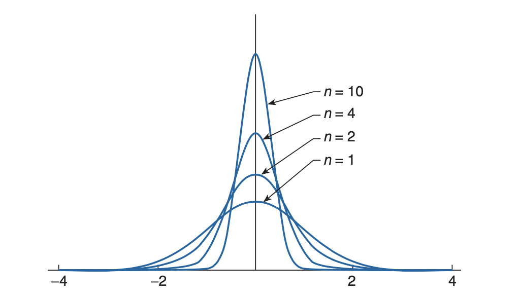
Corollary: Let $X_1,\dots,X_n$ be a sample from a normal population with mean $\mu$. If $\bar{X}$ denotes the sample mean and $S$ the sample standard deviation, then
\[\frac{\bar{X} - \mu}{S/\sqrt{n}} \sim t_{n-1}\]That is, $\sqrt{n}(\bar{X} - \mu)/S$ has a t-distribution with $n-1$ degrees of freedom.