
Perpetual student. Interested in Maths, Computer Science and Machine Learning.
Certain types of random variables occur over and over again in statistics. In this chapter, we will study a variety of them.
A random variable $X$, taking on one of the values $0, 1, 2,\dots,$ is said to be a Poisson random variable with parameter $\lambda, \lambda \gt 0$, if its probability mass function is given by
\[\begin{align} \prob(X=i) = e^{-\lambda}\frac{\lambda^i}{i!}, && i = 0,1, \dots \end{align}\]Both the mean and the variance of a Poisson random variable are equal to the parameter $\lambda$.
The Poisson random variable has a wide range of applications in a variety of areas because it may be used as an approximation for a binomial random variable with parameters $(n, p)$ where $n$ is large and $p$ is small. To see this, suppose that $X$ is a binomial random variable with parameters $(n, p)$ and let $\lambda = np$. Then
\[\begin{align} \prob(X = i) &= \frac{n!}{(n-i)!i!}p^i(1-p)^{n-i} \\ &= \frac{n!}{(n-i)!i!}\bigg(\frac{\lambda}{n}\bigg)^i\bigg(1 - \frac{\lambda}{n}\bigg)^{n - i} \\ &= \frac{n(n-1)\dots(n-i+1)}{n^i}\frac{\lambda^i}{i!}\frac{(1 - \lambda/n)^n}{(1 - \lambda/n)^i} \\\end{align}\]For $n$ large and $p$ small,
\[\begin{align} \bigg(1 - \frac{\lambda}{n}\bigg)^n &\approx e^{-\lambda} \\ \frac{n(n-1)\dots(n-i+1)}{n^i} &\approx 1 \\ \bigg(1 - \frac{\lambda}{n}\bigg)^i &\approx 1 \\ \end{align}\]Making these substitutions we get the equation for poission distribution
\[\begin{align} \prob(X=i) = e^{-\lambda}\frac{\lambda^i}{i!}, && i = 0,1, \dots \end{align}\]In other words, if $n$ independent trials, each of which results in a “success” with probability $p$, are performed, then when $n$ is large and $p$ small, the number of successes occurring is approximately a Poisson random variable with mean $\lambda = np$. This is called the Poisson approximation to the binomial variable.
A random variable is said to be normally distributed with parameters $\mu$ and $\sigma^2$, and we write $X \sim \mathcal{N}(\mu, \sigma^2)$, if its density is given by
\[f(x) = \frac{1}{\sqrt{2\pi}\sigma}e^{-(x-\mu)^2/2\sigma^2}\]The normal distribution was introduced by the French mathematician Abraham de Moivre in 1733 and was used by him to approximate probabilities associated with binomial random variables when the binomial parameter $n$ is large. This result was later extended by Laplace and others and is now encompassed in a probability theorem known as the Central Limit Theorem, which gives a theoretical base to the often noted empirical observation that, in practice, many random phenomena obey, at least approximately, a normal probability distribution.
An important fact about normal random variables is that if $X$ is normal with mean $\mu$ and variance $\sigma^2$, then $Y = \alpha X + \beta$ is normal with mean $\alpha \mu + \beta$ and variance $\alpha^2\sigma^2$.
It follows from the foregoing that if $X \sim \mathcal{N} (\mu, \sigma^2 )$, then
\[Z = \frac{X-\mu}{\sigma}\]is a normal random variable with mean $0$ and variance $1$. Such a random variable $Z$ is said to have a standard, or unit, normal distribution. Let $\Phi(·)$ denote its distribution function. That is,
\[\Phi(x) = \frac{1}{\sqrt{2\pi}}\int_{-\infty}^{x}e^{-y^2/2}dy\]This result that $Z = (X − \mu)/\sigma$ has a standard normal distribution when $X$ is normal with parameters $\mu$ and $\sigma^2$ is quite important, for it enables us to write all probability statements about $X$ in terms of probabilities for $Z$. For instance, to obtain $\prob(X < b)$, we note that $X$ will be less than $b$ if and only if $(X − \mu)/\sigma$ is less than $(b−μ)/σ$, and so
\[\begin{align} \prob(X < b) &= \prob\bigg\{\frac{X - \mu}{\sigma} < \frac{b - \mu}{\sigma} \bigg\} \\ &= \Phi\bigg(\frac{b-\mu}{\sigma}\bigg) \\ \end{align}\]Standard normal tables give us values of $\Phi(x)$ for non-negative $x$. We can obtain $\Phi(-x)$ from the table by making use of the symmetry of standard normal distribution around Y-axis.
\[\begin{align} \Phi(-x) &= \prob(Z < -x) \\ &= \prob(Z > x) & \mathrm{by\;symmetry} \\ &= 1 - \prob(Z < x) \\ &= 1 - \Phi(x) \\ \end{align}\]Definition For $\alpha \in (0, 1)$, let $z_\alpha$ be such that
\[\prob(Z > z_\alpha) = 1 - \Phi(z_\alpha) = \alpha \\\]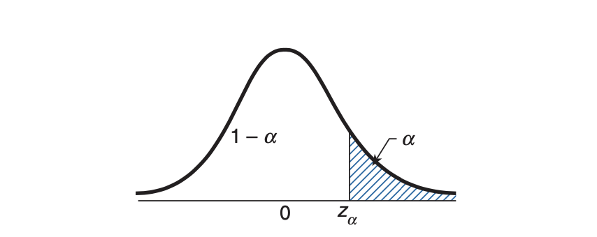
$X$ here is a normal random variable with mean $-\beta/2\alpha$ and variance $1/2\alpha$ .
All variables with distribution of the above form are normal distributions. You don’t really need to remember the mean and variance. Comparing the above equation with $f(x) = \frac{1}{\sigma\sqrt{2\pi}}e^{\frac{-(x-\mu)^2}{2\sigma^2}}$, we know that coefficient of $x^2 = \frac{1}{2\sigma^2} = \alpha$. Also, the mean is where the function takes the biggest value. That is the point where the absolute value of exponent of $e$ takes the smallest value. Differentiating the exponent function you get the mean.
If $Z_1, Z_2, \dots , Z_n$ are independent standard normal random variables, then $X$ , defined by
\[X = Z_1^2 + Z_2^2 + \dots + Z_n^2\]is said to have a chi-squared distribution with $n$ degrees of freedom. We will use the notation
\[X \sim \chi_n^2\]to signify that $X$ has a chi-square distribution with $n$ degrees of freedom.
The chi-square distribution has the additive property that if $X_1$ and $X_2$ are independent chi-square random variables with $n_1$ and $n_2$ degrees of freedom, respectively, then $X_1 + X_2$ is chi-square with $n_1 + n_2$ degrees of freedom.
If $X$ is a chi-square random variable with $n$ degrees of freedom, then for any $\alpha \in (0, 1)$, the quantity $\chi^2_{\alpha, n}$ is defined to be such that
\[\prob(X \geq \chi^2_{\alpha, n}) = \alpha\]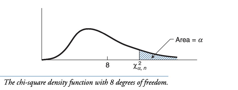
It is easy to prove that, for a chi-square variable with degree $n$
\[\expect[X] = n\]If $Z$ and $χ_n^2$ are independent random variables, with $Z$ having a standard normal distribution and $\chi_n^2$ having a chi-square distribution with $n$ degrees of freedom, then the random variable $T_n$ defined by
\[T_n = \frac{Z}{\sqrt{\chi^2_n/n}}\]is said to have a t-distribution with n degrees of freedom.
Like the standard normal density, the t-density is symmetric about zero. In addition, as $n$ becomes larger, it becomes more and more like a standard normal density. To understand why, recall that $\chi_n^2$ can be expressed as the sum of the squares of $n$ standard normals, and so
\[\frac{\chi^2_n}{n} = \frac{Z_1^2 + \ldots + Z_n^2}{n}\]where $Z_1,\ldots, Z_n$ are independent standard normal random variables. It now follows from the weak law of large numbers that, for large $n$, $\chi^2_n/n$ will, with probability close to $1$, be approximately equal to $E[Z_i^2] = 1$. Hence, for large $n$, $T_n = \frac{Z}{\sqrt{\chi^2_n /n}}$ will have approximately the same distribution as $Z$. A graph of the density function of $T_n$ is given below for $n = 1, 5$ and $10$.
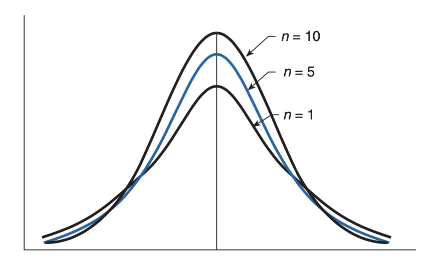
The t-density has thicker “tails,” indicating greater variability, than does the normal density. The mean and variance of $T_n$ can be shown to equal
\[\expect[T_n] = 0 \\ \v(T_n) = \frac{n}{n-2}\]For $\alpha$, $0 < \alpha < 1$, let $t_{\alpha, n}$ be defined so that
\[\prob(T_n \geq t_{\alpha, n}) = \alpha\]