
Perpetual student. Interested in Maths, Computer Science and Machine Learning.
Within the field of statistics there are two prominent schools of thought, with opposing views: the Bayesian and the Classical (also called Frequentist). Their fundamental difference relates to the nature of the unknown models or variables. In the Bayesian view, they are treated as random variables with known distributions. In the classical view, they are treated as deterministic quantities that happen to be unknown.
The Bayesian approach essentially tries to move the field of statistics back to the realm of probability theory. The unknown parameters are treated as random variables with known prior distrubtions. We conduct an experiment, make some observation ($X$) and then try to infer the value of the random variable ($\Theta$) during the conducted experiment. We derive a posterior distribution $\prob(\Theta \vert X)$ which tells us how likely it is that $\Theta = \theta$ when the observation $X$ was made.
Lecture 14, Intro to Probability
Here, we study the Bayes’ Rule in detail. We learn how to calculate the Posterior distribution and how to summarize the distribution using one number: either the most probable value (where posterior is highest) or the expected value (mean value).
In Bayesian Framework, the unknown quantity is modelled as a random variable, denoted by $\Theta$. It has a prior distribution $\prob_\Theta$. We aim to extract information about $\Theta$, based on another random variable observed during the experiment $X=(X_1, X_2, \dots, X_n)$. This random variable is called observation, measurement or an observation vector.
Based on $X$, we try to guess the value that $\Theta$ took during the experiment. For this we are given a model $\prob(X \vert \Theta)$. Once we have made an observation, we make a judgement about $\Theta$ by calculating posterior distribution $\prob(\Theta \vert X)$ using Bayes’ Rule.
$P(\Theta \vert X)$ is called the Posterior Distribution because here we have already made the observation and we are trying to go back and guess what value the random variable $\Theta$ took.
$P(X \vert \Theta)$ is called the Likelihood Distribution because it tells us how likely $X$ is to take a value $x$ (likelihood of data), given the value of $\Theta$.
$P(\Theta)$ is called the Prior Distribution, because it gives the probability of $\Theta = \theta$ before any observation is made. The prior comes from symmetry, known range, earlier studies, subjectivity etc.
Below is a list of the four different possible scenarios between continuous/discrete $\Theta$ and continuous/discrete $X$.
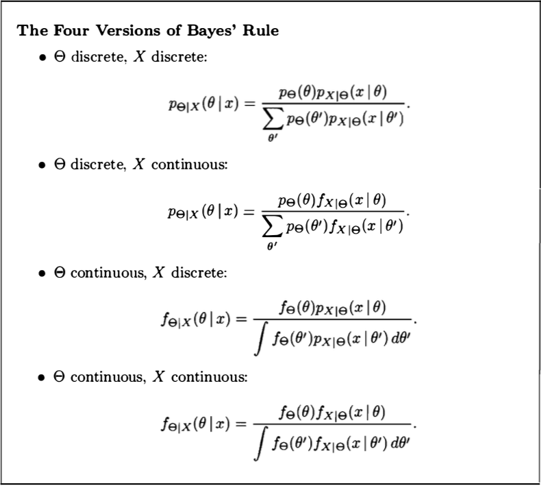
Let us look at a particular example where unknown is continuous and observation is discrete. We want to find the posterior probability of bias (probability of heads) of a coin, given the number of heads ($k$) in $n$ coin tosses. The formula for the posterior distribution is given above (continuous $\Theta$, discrete $X$ scenario). The prior $f_\Theta(\theta)$ is uniform over the interval $[0,1]$.
\[\begin{align} p_{K | \Theta}(k | \theta) &= \Comb{n}{k} \theta^k (1-\theta)^{n-k} \\ f_{\Theta | K}(\theta | k) &= \frac{1 \cdot \Comb{n}{k} \theta^k (1-\theta)^{n-k}}{p_{K}(k)} \\ &= \frac{1}{d(n,k)} \theta^k (1-\theta)^{n-k} \\ \end{align}\]$d(n,k)$ is the Normalizing Constant (doesn’t vary with $\Theta$). The distribution given by the above formula is called Beta distribution with parameters $(k+1, n-k +1)$. Notice that if we start with a Prior that is a Beta Distribution, then the Posterior still belongs to the Beta family. Priors of this sort are known as Conjugate Priors.
Many a times we are not interested in the posterior distribution of $\Theta$ over its entire range. We just need a point estimate for $\Theta$ given the value of $X$. Given a value of $X$ (say $x$), the point estimator takes a specific value based on the function $\prob(\Theta \vert X = x)$. Therefore, the point estimator itself is a random variable denoted by $\hat{\Theta}$. Any value that the point estimator takes is called an estimate and is denoted by $\hat{\theta}$.
The value of $\hat{\theta}$ is to be determined by applying some function $g$ to the observation $x$, resulting in $\hat{\theta} = g(x)$. The random variable $\hat{\Theta} = g(X)$ is called an estimator, and its realized value equals $g(x)$ whenever the random variable $X$ takes the value $x$. As explained, the reason that $\hat{\Theta}$ is a random variable is that the outcome of the estimation procedure depends on the random value of the observation.
We can use different functions $g$ to form different estimators; some will be better than others. For an extreme example, consider the function that satisfies $g(x) = 0$ for all $x$. The resulting estimator, $\hat{\Theta} = 0$, makes no use of the data, and is therefore not a good choice. We study two of the most popular estimators:
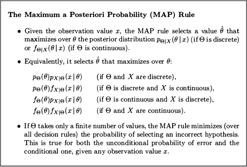
Maximum a Posteriori Probability (MAP) Estimator
Conditional Expectation Estimator
\[\hat{\theta} = \expect[\Theta \vert X=x]\]It is also called the least mean squares (LMS) estimator because it has an important property: it minimizes the Mean Squared Error over all estimators (proved in the next section).
If the posterior distribution is symmetric around its (conditional) mean and unimodal (i.e., has a single maximum), the maximum occurs at the mean. Then, the MAP estimator coincides with the conditional expectation estimator.
Watch this video for a nice summary of all the topics discussed in Lecture 14.
Lecture 16, Intro to Probability
So far we’ve seen two ways of estimating a parameter : maximum aposteriori estimation and conditional expectation. These were arbitrary choices. Here we will first decide upon a performance criterion and then find an estimator that is optimal with respect to that criterion. Our criterion will be the expected value of squared estimation error. It will turn out that the Conditional Expectation is the optimal estimator for this criterion. That is why we’ve been calling it Least Mean Squares Estimator all along.
Let us first consider the case where we don’t have any observation. Therefore we are trying to estimate $\Theta$ based on the prior distribution (the posterior is the same as the prior). Let us say the prior distibution is uniform in the interval $[4, 10]$. In this case, the MAP and Conditional Expectation estimators are given as follows:
MAP Rule : $\hat{\theta} \in [4, 10]$
Conditional Expectation : $\hat{\theta} = 7$
Instead of picking an estimator according to some arbitrary rule, let us find an estimator according to the following criterion:
\[\hat{\theta} = \textrm{arg}\min_{\hat{\theta}} \expect[(\Theta - \hat{\theta})^2]\]The expected value of $\Theta$ is the optimal estimator according to this criterion. Proof?
\[\begin{align} \expect[(\Theta - \hat{\theta})^2] &= \v(\Theta - \hat{\theta}) + (\expect[\Theta - \hat{\theta}])^2 \\ &= \v(\Theta) + (\expect[\Theta] - \hat{\theta})^2 &\hat{\theta}\textrm{ is a constant} \\ \end{align}\]We can’t reduce the variance of the random variable $\Theta$. We can only reduce the second term by setting $\hat{\theta} = \expect[\Theta]$.
Here again we want to find a point estimate $\hat{\theta}$ for the unknown variable $\Theta$ with prior $\prob_{\Theta}(\theta)$. But in this case, we also have an observation $X = x$. In the warm-up example, we wanted a point estimate that would minimize the squared estimation error, given by $\expect[(\Theta - \hat{\theta})^2]$. Here we would want to minimize the conditional mean squared error given by
\[\expect[(\Theta -\hat{\theta})^2 \vert X = x]\]As in the warm-up example, the solution is given by the expected value of $\Theta$, but now in the conditional universe.
\[\hat{\theta} = \expect[\Theta \vert X = x]\]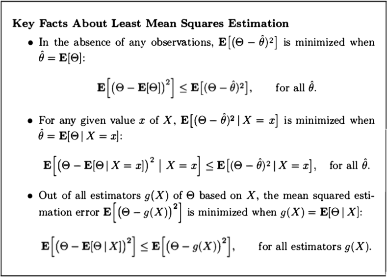
Given an observation $X=x$, we know that the optimal estimator for minimizing the criterion $\expect[(\Theta -\hat{\theta})^2 \vert X = x]$ is given by $\expect[\Theta \vert X =x ]$. We haven’t explicitly talked about the performance of our estimator with respect to our chosen criterion.
Expected performance when we already have a measurement:
\[\textrm{MSE} = \expect[(\Theta -\expect[\Theta \vert X = x])^2 \vert X = x] = \v(\Theta \vert X = x)\]What is the expected performance over all possible values of $X$? In this case the estimator is given as $\hat{\Theta} = \expect[\Theta \vert X]$
\[\begin{align} \textrm{MSE} &= \expect[(\Theta - \hat\Theta)^2] \\ &= \expect[\expect[(\Theta -\hat{\Theta})^2 \vert X]] &\textrm{Law of Iterated Expectations} \\ &= \expect[\v(\Theta \vert X)] &\textrm{Proved Above} \\ \end{align}\]