
Perpetual student. Interested in Maths, Computer Science and Machine Learning.
Lecture 11
Here we learn how to derive the distribution of a function of a random variable $Y = g(X)$, given the distribution of $X$ itself. We learn how to do that for discrete and continuous variables separately and then devise a common approach for both kinds using cummulative densities.
Note that the expected value of a function of random variable can be found out directly by using the formula:
\[\expect[g(X)] = \int_{-\infty}^{+\infty}g(x)p_X(x)dx\]What we study here is needed only in case we need the full distribution. Finally we learn how to find distribution for $Z = g(X,Y)$ given the joint distribution for $X$ and $Y$.
Discrete Random Variable
Suppose $Y = aX + b$. We need to find the PMF for $Y$.
\[\begin{align} p_Y(y) &= \prob(Y=y) \\ &= \prob(aX+b = y) \\ &= \prob(X = \frac{y-b}{a}) \\ &= p_X(\frac{y-b}{a}) \end{align}\]Thus,
\[Y = aX+b \implies p_Y(y) = p_X(\frac{y-b}{a})\]Continuous Random Variable
Here $F$ denotes the CDF. Let $Y = aX + b$ be the derived variable.
\[\begin{align} F_Y(y) &= \prob(Y \leq y) \\ &= \prob(aX+b \leq y) \\ &= \prob(X \leq \frac{y-b}{a}) & \text{when a > 0, inverse otherwise}\\ &= F_X(\frac{y-b}{a}) \end{align}\]Differentiating w.r.t. $y$ gives us,
\[f_Y(y) = \frac{1}{\mid a \mid}f_X(\frac{y-b}{a})\]This makes intuitive sense. The PDF graph of $Y=aX+b$ is the same as that of $X$, but only horizontally stretched by $a$ and translated horizontally by $b$. If we stretch a graph by $a$, the area under the graph also gets scaled by $a$. Therefore, in order to keep the area under the graph equal to $1$, we need to divide by $\mid a \mid$.
The above result also proves that, if $X \sim N(\mu, \sigma^2)$, then $aX +b \sim N(a\mu + b, a^2\sigma^2)$. It is very easy to prove using the formula above. In case you need help, refer to the slides.
We can use the above described technique (using CDF) to derive the distribution of any general function $g(X)$ (not necessarily linear). The two step procedure is as follows:
Now we will derive a general formula for the PDF of $Y = g(X)$, when $g$ is monotonic. Assume $g$ is strictly increasing and differentiable. Let $h$ be the inverse function of $g$. Then,
\[\begin{align} F_Y(y) &= \prob(Y \leq y)\\ &= \prob(X \leq h(y)) & \textrm{ because of monotonicity} \\ &= F_X(h(y)) \\ \therefore f_Y(y) &= f_X(h(y)) |\frac{dh}{dy}(y)| \end{align}\]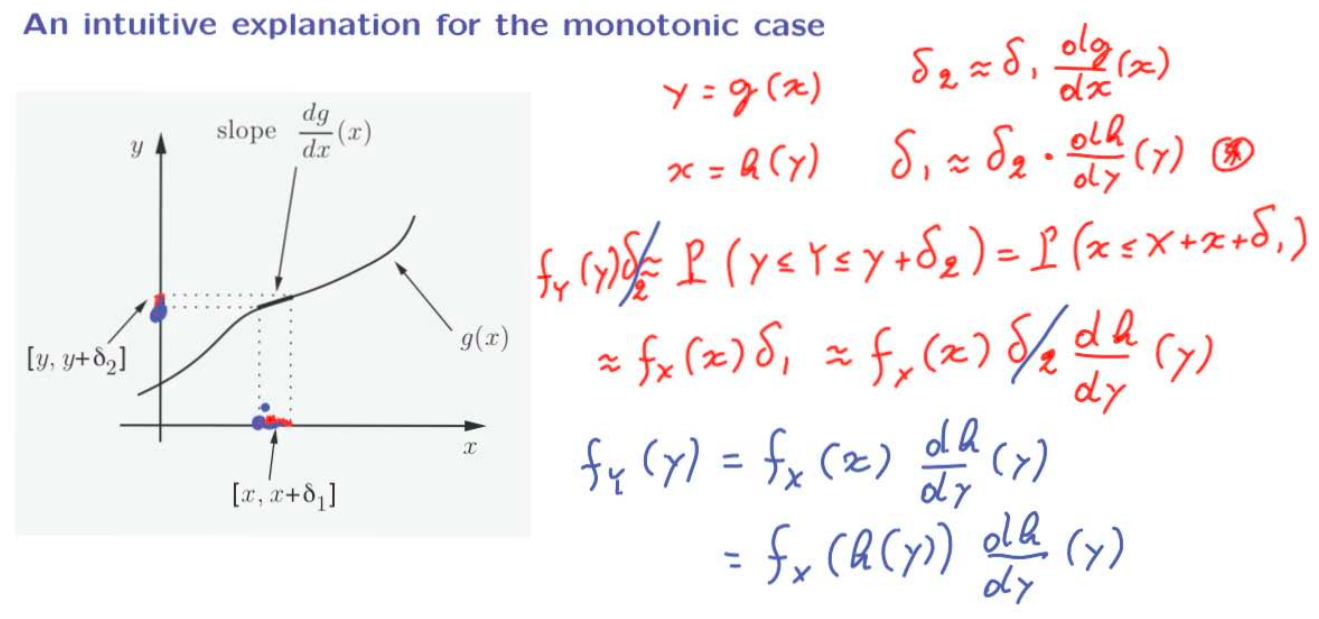
Till now we have considered the case where $Y$ is a function of $X$ (linear / monotonic / non-monotonic). What if the random variable of interest $Z$ is a function of two independent random variables $X$ and $Y$? How do we calculate the PDF of $Z = g(X,Y)$ in that case? The method remains the same. We use the joint probability distribution of $X$ and $Y$ to somehow find the CDF of $Z$. Then we differentiate the CDF to find the PDF of $Z$. See Lec 11.9 for an example of the same.
Lecture 12
Here we see how to calculate the PMF/PDF of $X + Y$ when $X$ and $Y$ are independent variables (continuous and discrete) and specifically when $X$ and $Y$ are independent normals ($X+Y$ is also a normal in this case). These are all special cases of the $Z=g(X,Y)$ scenario studied in Derived Distributions. Finally we study covariance and correlation. Covariance and Correlation play an important role in predicting value of one random variable, given another random variable (machine learning).
The Discrete Case
The PMF of $Z = X + Y$, when $X$ and $Y$ are independent and discrete, is given by:
\[\prob_Z(z) = \sum_x\prob(X=x,Y=z-x) = \sum_x\prob_X(x)\prob_Y(z-x)\]The above operation, of deriving the distribution of the sum of two random variables, is known as convolution of those random variables.
How do you calculate the value of convolution for a given value of $Z$ (denoted by $z$)? You flip (horizontally) the PMF of $Y$. Then shift it to the right by $z$. Finally, element wise cross mutliply the derived PMF with the PMF of $X$ and add each term together. This will give you the value of $\prob_Z$ for one specific $z$.
The Continuous Case
The convolution of continuous independent random variables $X$ and $Y$ is given by:
\[f_Z(z) = \int_{-\infty}^{+\infty}f_X(x)f_Y(z-x)\,dx\]The mechanics of calculating the convolution are the same for the continuous case (flip, shift, etc.)
Let us now come to the specific case where $X$ and $Y$ are independent normal variables. Let $Z = X + Y$.
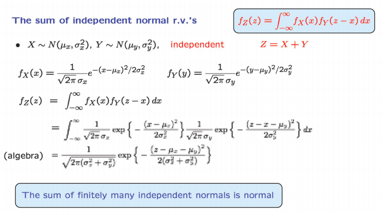
Thus, $Z$ is also a normal variable with mean $\mu_x + \mu_y$ and variance of $\sigma_x^2 + \sigma_y^2$. The mean and variance can also be derived easily using the Linearity of Expected Values and Linearity of Variances for Independent Variables.
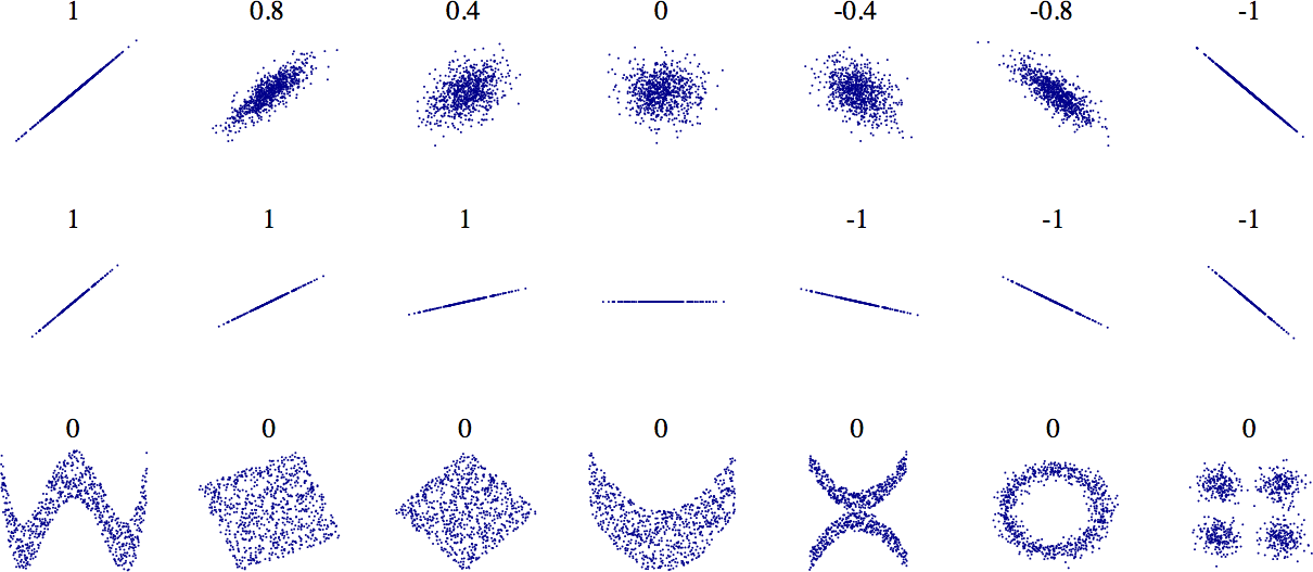
Covariance basically tells us if two variables $X$ and $Y$ vary in the same or different directions from their respective means. Positive Covariance indicates that $X$ and $Y$ go above/below their respective means simultaneously. Negative Covariance indicates that when $X$ goes above its mean, $Y$ goes below, and vice-versa.
\[\cov(X,Y) = \expect[(X - \expect[X])(Y - \expect[Y])]\]If $X$ and $Y$ are zero-mean random variables, then covariance is given by $\expect[XY]$. If both $X$ and $Y$ increase and decrease in tandem, then the values of $X$ vs $Y$ graph will lie in first and third quadrant and the covariance will be positive. If $Y$ decrease when $X$ increase and vice-versa, then the values will lie in second and forth quadrant and the covariance will be negative. If the two random variables are independent, then the covariance becomes \(\expect[XY] = \expect[X]\expect[Y] = 0\cdot 0 = 0\)
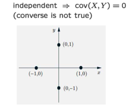
The covariance of independent variables is always zero, but variables whose covariance is zero are not always independent. In the figure below, it is evident that the covariance is zero (either $X$ or $Y$ is zero $\implies$ $E[XY] = 0$) . However, the two variables are not independent. Knowing that $X=1$ tells us that $Y=0$.
Properties
Correlation is the dimensionless version of covariance. The sign of covariance shows if two variables move away from their respective means in the same direction or different. But it is hard to make sense of the magnitude of covariance. Correlation is defined as an alternative :
\[\rho(X,Y) = \expect\Bigg[\frac{X-\expect[X]}{\sigma_X}\times\frac{Y-\expect[Y]}{\sigma_Y}\Bigg] = \frac{\cov(X,Y)}{\sigma_X\sigma_Y}\]Notice that the correlation coefficient is the expected value of the product of z-scores of $X$ and $Y$. More on z-scores in a minute.
Property 1:
An important property of the correlation coefficient is that it always lies between $-1$ and $1$.
\[-1 \leq \rho \leq 1\]This allows us to judge whether a given correlation coefficient is small or large (because now we have an absolute scale). Therefore, it provides us a measure of the degree of “association” between $X$ and $Y$. Proof?
If $X$ and $Y$ have zero means and unit variances, then
\[\begin{align} 0 \leq \expect[(X-\rho Y)^2] &= E[X^2] - 2 \rho \expect[XY] + \rho^2\expect[Y^2]\\ &= 1 - 2 \rho^2 + \rho^2\\ &= 1 -\rho^2\\ \end{align}\]Thus, $\rho^2 \leq1$. All this can also be proved if $X$ and $Y$ don’t have unit variance and zero mean, using somewhat more involved calculations.
Also, notice that if $\rho = \pm1$, then $X = \rho Y$, which means $X$ is a linear function of $Y$.
Property 2:
When $X$ and $Y$ are independent, $\cov(X, Y) = 0 \implies \rho(X,Y) = 0$ (converse is not true).
Property 3:
We just considered the case where $X$ and $Y$ are independent. Now we look at the other extreme case, where $X$ and $Y$ are as dependent as they can be, i.e. $Y = X$:
\[\rho(X,X) = \frac{\v(X)}{\sigma_X^2} = 1\]Property 4:
\[\cov(aX + b, Y) = a\,\cov(X, Y) \implies \rho(aX+ b, Y) = \frac{a\,\cov(X, Y)}{|a|\sigma_x\sigma_y} = \textrm{sign}(a)\,\rho(X, Y)\]Thus, unlike co-variance, correlation is not affected by linear stretching or contraction. This is an important property that makes correlation meaningful.
Property 5:
Combining properties 3 and 4, we can conclude that if $Y = aX + b$, then $\rho(X, Y) = \pm 1$. The correlation coefficient is $\pm 1$, if the variables are linearly related.
\[\mid\rho\mid = 1 \Leftrightarrow (X-\expect[X]) = c(Y-\expect[Y])\]Refer to Lec 12.10 and 12.11 for intuition behind correlation and its practical use. Remember that correlation coefficient can only measure linear dependence between variables. The variables might be dependent (non-linearly) and have correlation coefficient of zero.
Standard scores (also known as z-scores) give us a way of comparing values across different data sets even when the sets of data have different means and standard deviations. They’re a way of comparing values as if they came from the same set of data or distribution. As an example, you can use standard scores to compare each player’s performance relative to his own personal track record—a bit like a personal trainer would.
Standard scores work by transforming sets of data into a new, theoretical distribution with a mean of 0 and a standard deviation of 1. It’s a generic distribution that can be used for comparisons. Standard scores effectively transform your data so that it fits this model while making sure it keeps the same basic shape.
Standard scores can take any value, and they indicate position relative to the mean. Positive z-scores mean that your value is above the mean, and negative z-scores mean that your value is below it. If your z-score is 0, then your value is the mean itself. The size of the number shows how far away the value is from the mean.
Standard Score = Number of Standard Deviations from the Mean
Generally, values that are more than three standard deviations away from the mean (z-score > 3) are known as outliers.
Lecture 13
We will study how conditional expectations and conditional variances can be treated as random variables. $\expect[X \mid Y]$ is a function of $Y$ and thus is itself a random variable. Then we use that knowledge to calculate the expectation and variance of the sum of random number of independent variables.
Let $g(Y)$ be a random variable that takes the value $\expect[X \mid Y=y]$, if $Y$ happens to take the value $y$.
\[\begin{align} g(y) &= \expect[X \mid Y=y] \\ g(Y) &= \expect[X \mid Y] \\ \expect[g(Y)] &= \expect[\expect[X \mid Y]] \\ \end{align}\]The mean of $E[X \mid Y]$ is given by the Law of Iterated Expectations, which says:
\[\expect[\expect[X \mid Y]] = \expect[X]\]In Lec 13.4 we use Law of Iterated Expectations to solve the stick breaking problem.
$\v(X \mid Y)$ is the random variable that takes the value $\v(X \mid Y=y)$, when $Y= y$.
Law of Total Variance says:
\[\v(X) = \expect[\v(X \mid Y)] + \v(\expect[X \mid Y])\]In order to get an intuitive understanding of the Law of Total Variance, we consider the example problem of Section Means and Variances. We divide the entire set of students (sample space) into multiple sections. The experiment is to pick a student at random. Random variable $X$ denotes the marks of that student and random variable $Y$ denotes the section of that student.
Here, $\expect[X \mid Y]$ gives the average score of a student in one particular section and $\v(X\mid Y)$ gives the variation in the marks of the students for a particular section. We find the following alternate way of looking at law of total variance:
Here we learn how to find the mean and variance of the sum of a random number of independent random variables. Let $N$ be a random variable denoting the number of stores visited, and let $X_1, X_2, \dots X_n$ be the money spent at each store. All the $X_i$s are independent identically distributed random variables. They are also independent of $N$. We want to derive details of the random variable $Y$ such that \(Y = \sum_iX_i\)
\[\begin{align} \expect[Y \mid N=n] &= \expect[X_1 + \dots + X_N \mid N = n] \\ &= \expect[X_1 + \dots + X_n \mid N = n] \\ &= \expect[X_1 + \dots + X_n] \\ &= n\expect[X] \end{align}\]Now, Total Expectation Theorem says that:
\[\expect[Y] = \sum_n \bigg(p_N(n)\expect[Y \mid N=n] \bigg) = \sum_n\bigg( p_N(n)\;n\; \expect[X]\bigg) = \expect[N]\;\expect[X]\]This can also be derived using Law of Iterated Expectations:
\[\expect[Y] = \expect[\expect[Y \mid N]] = \expect[N\expect[X]] = \expect[N]\expect[X]\]Total Variance of $Y$ can be derived using Law of Total Variance. The derivation is simple and mundane.
When working with multiple variables, the covariance matrix provides a succinct way to summarize the covariances of all pairs of variables. If $\mathbf{X} = (X_1, \dots, X_n)^T$ is a $n \times 1$ multivariate random variable, then the covariance matrix, which we usually denote as $\Sigma$, is the $n \times n$ matrix whose $(i, j)$th entry is $\cov(X_i, X_j)$.
\[\begin{equation} \underset{n\times n}{\Sigma}=\left(\begin{array}{cccc} \sigma_{1}^{2} & \sigma_{12} & \cdots & \sigma_{1n}\\ \sigma_{12} & \sigma_{2}^{2} & \cdots & \sigma_{2n}\\ \vdots & \vdots & \ddots & \vdots\\ \sigma_{1n} & \sigma_{2n} & \cdots & \sigma_{n}^{2} \end{array}\right) \end{equation}\]Refer to Chapter 3.6 of Bookdown.org for more details. Of particular importance is section 3.6.6, which states that:
If $\mathbf{Y} = \mathbf{AX} + \mathbf{b}$, then $\Sigma_\mathbf{Y} = \mathbf{A}\Sigma_\mathbf{X}\mathbf{A}^T$.
Notice that if $X_1, \dots, X_n$ are all independent random variables, then $\Sigma_\mathbf{X}$ is a diagonal matrix.
We saw that if $X$ and $Y$ are independent normal variables then
\[\begin{align} f_{X, Y}(x,y) &= \frac{1}{2\pi \sigma_x \sigma_y }\textrm{exp}\bigg\{-\frac{(x-\mu_x)^2}{2\sigma_x^2}-\frac{(y-\mu_y)^2}{2\sigma_y^2}\bigg\} & (1) \\ \end{align}\]If we consider \(\bt{X} = \mat{X \\ Y}\), then we can rewrite the above equation as
\[\begin{align} f_\bt{X}(\bt{x}) &= \frac{1}{2\pi \sigma_x \sigma_y }\textrm{exp}\bigg\{-\frac{1}{2}(\bt{x} - \bt{\mu})^T\Sigma^{-1}(\bt{x} - \bt{\mu})\bigg\}\\ &= \frac{1}{ (2\pi)^{n/2} |\Sigma|^{1/2} } \textrm{exp}\bigg\{-\frac{1}{2}(\bt{x} - \bt{\mu})^T\Sigma^{-1}(\bt{x} - \bt{\mu})\bigg\} & (2)\\ \end{align}\]where $n$ is the num of independent variables. Intuitively, this makes sense: the smaller the variance of some random variable $X_i$, the more “tightly” peaked the Gaussian distribution in that dimension.
Unfortunately, this derivation is restricted to the case where these entries are independent and 0-centered. How do we generalize to the case of Multivariate Gaussian Distribution with a non-diagonal covariance matrix? There are two ways to look at this:
Noah Golmant Blog (Part 2) takes the first approach and CS229 Handout (Appendix A.2) takes the second approach. The proofs also show that the affine transformation specifically consists of a rotation followed by a scaling along the principal axes of the rotation, with one translation.
Side Note: The fact that two random variables $X$ and $Y$ both have a normal distribution does not imply that the pair $(X, Y)$ has a joint normal distribution. See details.