
Perpetual student. Interested in Maths, Computer Science and Machine Learning.
Lecture 05
In this section we go over what Discrete Random Variables are, and how we calculate their Probability Mass Functions. Then we look at a few common types of Discrete Random Variables, specifically Uniform, Bernoulli, Binomial and Geometric Random Variables. Finally we learn about Expected Values and their properties.
A Random Variable (RV) associates a value (a number) to every possible outcome of an experiment. Mathematically, it is a function from the sample space $\Omega$ to the set of real numbers $\R$. It can take discrete or continuous values. We can have several random variables defined on the same sample space. That is, there can be multiple ways of mapping the outcomes of the same experiment to the number line. All these different ways constitute different random variables. A function of one or several random variables is also a random variable , like $X + Y$.
Probability Mass Function (PMF) is the “probability law” or “probability distribution” of a discrete random variable.
\[p_X(x) = \prob(X=x) = \prob(\{ \omega \in \Omega \text{ s.t. } X(\omega) = x\})\]Examples of Discrete Random Variables
Bernoulli Random Variable models a trial that results in success/failure. It is used to indicate whether an event $A$ occurred or not. Therefore, it is also called an indicator random variable.
Binomial Random Variable represents the total number of heads when a coin is flipped multiple times with probability $p$ of getting heads in each toss. If $X$ is a binomial variable and $k$ is the number of heads achieved in $n$ coin tosses, then
How do both the definitions lead to the same measure? Is it necessary that the frequencies in a large population will follow the probability distribution? Is the probability (likelihood) of an observation the same as its frequency when the experiment is conducted a large number of times? The intuition is easy to catch if we look at probabilities as frequencies. The mathematical proof is given by the Weak Law of Large Numbers (studied later in the note on Limit Theorems).
Consider an experiment where we randomly pick a student in a classroom of $n$ students. The weight of the $i^{th}$ student is $x_i$. If the variable $X$ is defined as the weight of the selected student, then $p_X(x_i) = \frac{1}{n}$ and the expected value is
\[E(X) = \sum_i x_i p_X(x_i) = \frac{1}{n} \sum_i x_i\]Thus, in this case, the expected value (which is the average of observations over multiple runs of the experiment) is equal to the population average (mean weight of a student in the class).
Properties of Expectations:
$\quad\quad$ Proof? Let $Y = aX + b = g(X)$. Then,
\[\begin{align} E[Y] &= \sum_x g(x)p_X(x) \\ &= \sum_x (ax + b)p_X(x) \\ &= a\sum_x xp_X(x) + b\sum_x p_X(x) \\ &= aE[X] + b\\ \end{align}\]Lecture 06
Expected Value gives an average (central tendency) of the probability distribution. But how do you measure the spread of the distribution?
One way to measure the spread is the range (highest possible value - lowest possible value). But this is severely affected by outliers. Thus, other measures like Quartiles and Percentiles are often used. Percentiles give us the flexibility of discounting as many outliers as required. However these measures still don’t tell us how the observations are distributed around the mean value. How do you measure how close are the actual observations to the Expected Value? The solution is given by Variance.
Variance measures the average squared distance of a Random Variable from the Expected Value (over multiple trials). It quantifies the amount of randomness that is present. Together with the expected value, the variance summarizes crisply the properties of a PMF.
\[\v(X) = \expect[(X-\mu)^2] \\ \textbf{standard deviation} : \sigma_X = \sqrt{\v(X)}\]Properties of Variance:
$\v(aX+b) = a^2\v(X)$
$\v(X) = \expect[X^2] - (\expect[X])^2$
Proof?
\[\begin{align} \v(X) &= \expect[(X - \mu)^2] \\ &= \expect{[X^2 - 2X\mu + \mu^2]} \\ &= \expect[X^2] -2\mu\expect[X] + \mu^2 \\ &= \expect[X^2] -2\mu\expect[X] + \mu^2 \\ &= \expect[X^2] - (\expect[X])^2 \end{align}\]If $X$ is a Uniform RV with values between $a$ and $b$, then the $\expect[X] = \frac{a+b}{2}$ and $\v(X) = \frac{1}{12}(b-a)(b-a+2)$
If $X$ is a Bernoulli RV with probability $p$ of success, then $\expect[X] = p$ and $\v(X) = p(1-p)$
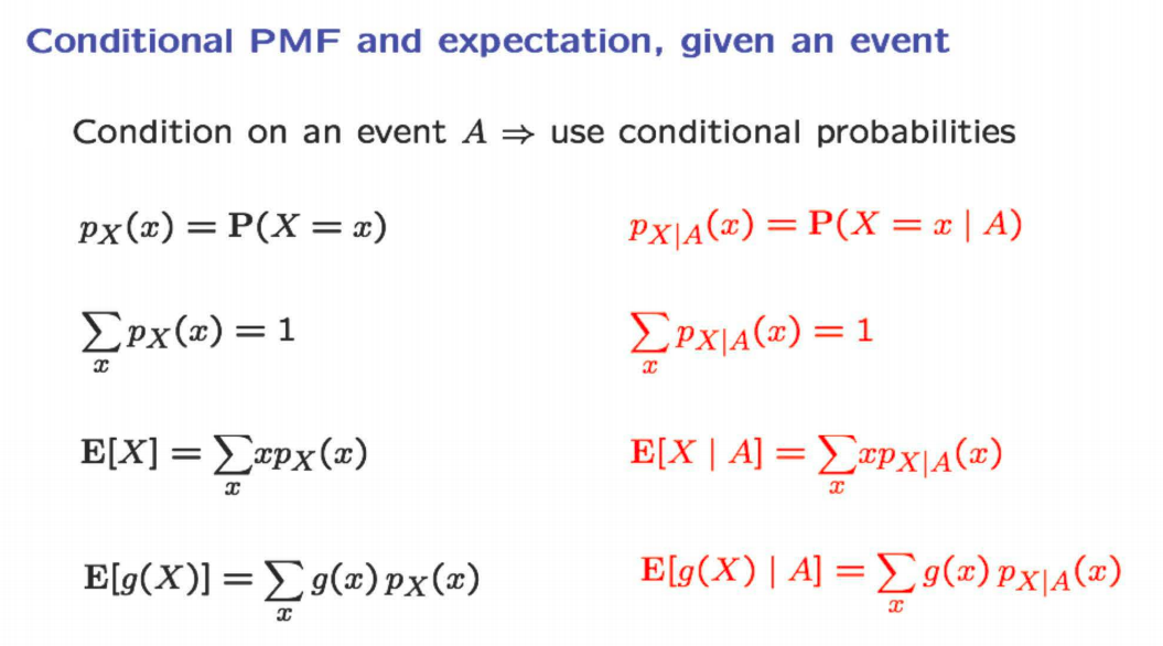
Here we discuss conditional PMF, conditional expected value and conditional variance (all conditioned on any event $A$). All the formulas remain the same, but now we use conditional probabilities instead of absolute probabilities.
Total Expectation Theorem
Total Expectation Theorem helps us divide and conquer expected value calculations. It states that
\[\expect[X] = \prob(A_1)\expect[X \mid A_1] + \dots + \prob(A_n)\expect[X \mid A_n]\]Let $X$ be a geometric random variable denoting the first heads in a series of coin tosses. Suppose the information that the first coin toss is tails ($X > 1$) is given. Then the remaining coin tosses (till the first heads) is given by the random variable $Y = X - 1$. Memorylessness Property states that the number of remaining coin tosses till the first heads, conditioned on tails in the first toss, is Geometric, with parameter $p$. For example, suppose the probability of getting the first head on third toss is $k$. If we get a tail on the first toss, then (given this fact) the probability of getting a head on the overall fourth toss (third remaining toss) is also $k$.
\[\begin{align} \prob_{X-1|X > 1}(a) &= \prob_{X}(a)\\ &\textbf{OR}\\ \prob_{X|X > 1}(a) &= \prob_{X}(a-1)\\ \end{align}\]Using this property we can derive the Expected Value of a Geometric Random Variable $X$.
\[\begin{align} \expect[X] &= 1 + \expect[X-1] \\ &= 1 + p\expect[X-1 \mid X=1] + (1-p)\expect[X-1 \mid X>1] \\ &= 1 + 0 + (1-p)\expect[X] \\ &= \frac{1}{p} \\ \end{align}\]Joint PMF of two different random variables $X$ and $Y$ is given by:
\[p_{X,Y}(x,y) = \prob(X=x \textrm{ and } Y=y)\]The following properties are obvious:
\[\begin{align} &\sum_{x}\sum_{y}p_{X,Y}(x,y) = 1 \\ &p_X(x) = \sum_y p_{X,Y}(x,y) \\ &p_Y(y) = \sum_x p_{X,Y}(x,y) \\ &\expect[g(X,Y)] = \sum_x \sum_y g(x,y)p_{X,Y}(x,y) \\ \end{align}\]Using the above properties, we can prove the linearity of expectation over multiple random variables.
\[\expect[X+Y] = \expect[X] + \expect[Y]\]Here $X$ and $Y$ don’t need to be independent.
The above property can be used to derive the Expected Value of a Binomial Random Variable $X$ with $n$ trials and $p$ probability of success. Let $X_i$ denote the result of $i^{th}$ trial. Then,
\[\begin{align} X &= X_1 + X_2 + \dots + X_n \\ \implies \expect[X] &= \expect[X_1] + \expect[X_2] + \dots +\expect[X_n] \\ &= p + p + \dots + p \\ &= np \\ \end{align}\]Lecture 07
In this part, we study conditioning of random variables on other random variables (as opposed to events, which we studied in last lecture). This is mainly just new notations and very straight-forward extension of concepts of joint PMF and conditionality. Then we introduce independence of random variables. We study the properties of expectations and variances for independent random variables. Finally, we study the Hat Problem and try to solve it using the tools we’ve developed so far.
We have studied conditional probability of a random variable given an event (in the previous lecture). We also studied the Joint PMF of two different random variables. Now we study conditional probability of a random variable given value of another random variable.
\[p_{X \mid Y}(x \mid y) = \frac{p_{X,Y}(x,y)}{p_Y(y)}\]Most conditional identities translate as is for PMF conditioned on another random variable:
\[\begin{align} \expect[X \mid Y = y] &= \sum_x x p_{X \mid Y}(x \mid y) \\ \expect[X] &= \sum_y p_{Y}(y) \expect[X\mid Y = y] \end{align}\]Two random variables $X$ and $Y$ are said to be independent if and only if
\[\begin{align} p_{X, Y}(x, y) &= p_X(x)p_Y(y) &\forall x, y \\ \end{align}\]Equivalently, we can say that
\[\begin{align} p_{X \mid Y}(x \mid y) &= p_X(x) \\ \textbf{and} \\ p_{Y \mid X}(y \mid x) &= p_Y(y) & \forall x, y\\ \end{align}\]if and only if $X$ and $Y$ are independent random variables.
Properties of Independent Random Variables:
$\expect[X + Y] = \expect[X] + \expect[Y]$ for all random variables, but only for independent random variables:
$ \expect[XY] = \expect[X] \times \expect[Y]$
Proof?
\[\begin{align} \expect[XY] &= \sum_x\sum_y x\,y\,p_{X,Y}(x,y) \\ &= \sum_x\sum_y x\,y\,p_{X}(x)\,p_{Y}(y) \\ &= \sum_x \bigg[x\,p_{X}(x) \bigg(\sum_y y\,p_{Y}(y)\bigg)\bigg] \\ &= \bigg(\sum_y y\,p_{Y}(y)\bigg) \bigg( \sum_x x\,p_{X}(x) \bigg) \\ &= \expect[X] \times \expect[Y] \end{align}\]$\v(X + Y) = \v(X) + \v(Y)$
Proof? To simplify the proof, we make the assumption that $X$ and $Y$ are zero-centered, i.e. $\expect[X] = \expect[Y] = 0$.
\[\begin{align} \v(X + Y) &= \expect[(X + Y)^2] \\ &= \expect[X^2 + 2XY +Y^2] \\ &= \expect[X^2] + \expect[2XY] + \expect[Y^2] \\ &= \expect[X^2] + 2\expect[X] \expect[Y] + \expect[Y^2] \\ &= \v(X) + \v(Y) \\ \end{align}\]The second property can be used to derive the variance of a Binomial Random Variable $X$ with $n$ trials and $p$ probability of success. Let $X_i$ denote the result of $i^{th}$ trial. Then,
\[X = X_1 + X_2 + \dots + X_n\]Now, $\v(X_i) = p(1-p)$. Therefore, given that all $X_i$(s) are independent of each other
\[\v(X) = \v(X_1) + \dots + \v(X_n) = np(1-p)\]In the hat problem, $n$ people throw their hats in a box and then pick one at random. At the time of retrieving hats, all permutations of the hats are equally likely. Let $X$ be a random variable, denoting the number of people who get their own hat back. We want to find the $\expect[X]$.
Let $X_j$ be the indicator variable for the event where person $j$ gets his own hat. Now there are $n!$ permutations in which the hats may be distributed. In them $(n-1)!$ ways give the correct hat to $j^{th}$ person. So the person $j$ gets his correct hat with the probability $\frac{(n-1)!}{n!}$ which is $\frac{1}{n}$.
Also there is some subtlety involved here. First the random variable $X$ (denoting total num of men receiving their own hat) and random variables $X_1, X_2, X_3, \dots, X_n$ etc. all map the outcomes of the same experiment to the number line. The experiment is that each person is assigned a hat. $X_i$ takes each hat permutation and assigns it $1$ if the $i$-th person received his own hat. $X$ takes each hat permutation and assigns it $k$ if in all $k$ people got their hat back.
Secondly, $X_1, X_2, X_3$ are all dependent on each other. If $X_1 \dots X_n$ all get their correct hats, $X_n$ automatically gets the correct hat.
Now, how do we find $\expect[X]$? We use the Linearity of Expected Value theorem.
\[\begin{align} X &= X_1 + X_2 + \dots + X_n \\ \implies \expect[X] &= \expect[X_1] + \expect[X_2] + \dots + \expect[X_n] \\ &= \frac{1}{n} + \frac{1}{n} + \dots + \frac{1}{n} &\textrm{as each }X_i\textrm{ is a Bernoulli RV with }p=\frac{1}{n} \\ &= 1 \\ \end{align}\]How do we find the variance of $X$? Here we can’t use Linearity of Variance, because $X_i$(s) are not independent. We will use the formula $\v(X) = \expect[X^2] - (\expect[X])^2$. The $\v(X)$ comes out to be $1$. Refer to Lec 07.8 for exact calculation.