
Perpetual student. Interested in Maths, Computer Science and Machine Learning.
Lecture 08
We study continuous random variables and their probability density functions. PDFs replace PMFs from the discrete case. We then study expected values and variances of continuous random variables. We also look at Cumulative Density Functions and then study common types of continuous distributions, namely Uniform, Exponential and Normal Distributions.
Probability Density Function (PDF) of a continuous random variable represents the probability density (probability per unit length) near each value of the random variable. PDF of a Random Variable $X$ is denoted by $f_X(x)$.
\[\prob(a \leq X \leq a + \delta) = f_X(a)\cdot\delta\]Thus $f_X(a)$ gives the probability of the $X$ lying in a very very small interval close to $a$ per unit length. It is important to understand that even though PDF is used to calculate event probabilities, $f_X(a)$ is not the probability of any particular event $a$. Also $f_X(x)$ is not less than or equal to one for all $ x \in \mathbb{R}$. Rather,
\[\int_{-\infty}^{+\infty}f_X(x)dx = 1\]Notice that by taking $\delta = 0$, we get
\[\prob(X=x) = 0\]This tells us that at any single point, the probability is exactly zero. Why? If $X$ denotes height of a person, then can’t we say that the height of a person is 180.5 cms with certainty? The thing to notice here is that even in the previous statement, we are specifying a range. The range covers all the double, triple, and higher precision floating points greater than 180.5 and less than 180.6.
The interpretation of expected values is still the same. It is the average of the random variable in large number of independent repetitions of the experiment.
Properties:
Variance is exactly similar to its discrete counterpart.
\[\begin{align} &\v(X) = \expect[(X - \mu)^2] \\ &\v(aX+b) = a^2\v(X) \\ &\v(X) = \expect[X^2] - (\expect[X])^2 \\ \end{align}\]Examples:
Below we introduce the Uniform and Exponential Continuous RVs. The derivations don’t introduce any new techniques and can be safely skipped over.
If $X$ is uniform between $a$ and $b$, then:
\[\begin{align} f_X(x) &= \frac{1}{b-a} &(a\leq x \leq b)\\ \end{align}\]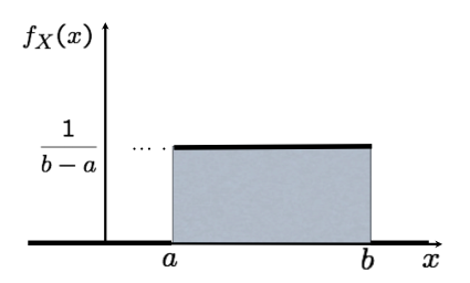
If $X$ is an exponential random variable with parameter $\lambda > 0$, then:
\[f_X(x) = \begin{cases} \lambda e^{-\lambda x} &x\geq0\\ 0 &x<0\\ \end{cases}\]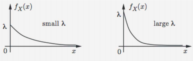
This is a concept that can be used to describe both, probability laws for discrete as well as continuous random variables. The value of CDF at a point $x$ is equal to the probability of $X$ being less than or equal to $x$. CDF is a non-decreasing function; and as $x \to +\infty$, $F_X(x) \to 1$.
The General Normal Distribution has two parameters $\mu$ and $\sigma^2$. If $X$ is a Normal Variable with parameters $\mu$ and $\sigma^2$, it is denoted as $X = N(\mu,\sigma^2)$ and the PDF of $X$ is as follows:
\[f_X(x) = \frac{1}{\sigma\sqrt{2\pi}}e^{-\frac{(x-\mu)^2}{2\sigma^2}}\]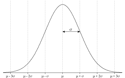
It is evident from the PDF equation that the distribution is symmetric around $\mu$. Thus, $\expect[X] = \mu$.
Using integration by parts it can be proved that $\v(X) = \sigma^2$ ($\sigma$ is the standard deviation of the distribution). We don’t prove it mathematically, but the formula seems intuitively coherent. We can see from the Normal PDF formula that if $\sigma$ increases, the graph becomes wider. This is coherent with standard deviation definition, which says that if s.d. increases, values move away from the mean.
$X = N(0,1)$ is called the Standard Normal Distribution. The simplified equation for Standard Normal is given below:
\[f_X(x) = \frac{1}{\sqrt{2\pi}}e^{-\frac{x^2}{2}}\]Finally, let us talk about linear functions of a Normal Random Variable. Let $X = N(\mu,\sigma^2)$ and $Y = aX + b$. We know that,
\[\begin{align} \expect[Y] = a\mu + b \\ \v[Y] = a^2\sigma^2 \end{align}\]We will prove later (in the section on ‘Derived Distributions’) that $Y$ is also a Normal Variable.
\[Y = N(a\mu + b, a^2\sigma^2)\]The CDF of a Standard Normal is given as follows:
\[F_X(x) = \int_{-\infty}^x\frac{1}{\sqrt{2\pi}}e^{-\frac{x^2}{2}}\, dx\]This equation doesn’t have any closed form solution. Fortunately, we do have tables for calculating cumulative densities of normal variables. For details about using these Standard Normal Tables, refer to Lec 8.9.
Lecture 09
We know that the PDF for a continuous random variable $X$, is defined by the following mathematical equation:
\[f_X(x)\cdot\delta = \prob(x\leq X \leq x+\delta)\]If we move to a conditional universe, where event $A$ is know to have occurred, then the probabilities of these intervals will be determined by conditional PDFs, given as follows:
\[f_{X \mid A}(x)\cdot \delta = \prob(x\leq X \leq x+\delta \mid A)\]Following are some analogies from the discrete variable case:
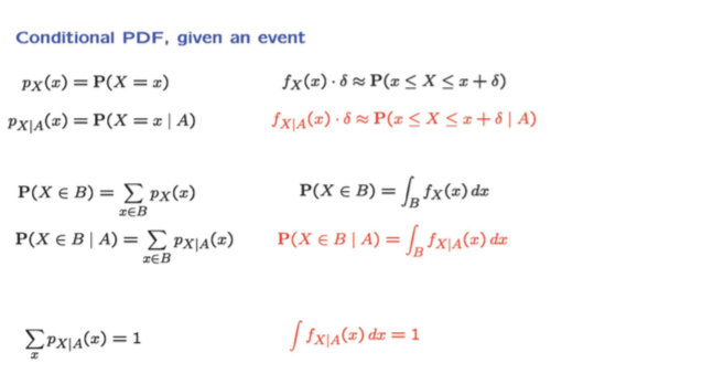
Let us condition on the special event where $X$ takes value in a certain set/interval $A$. Conditional PDF of $X$ given $X \in A$ is defined as follows:
\[f_{X|X\in A}(x) = \begin{cases} 0 & x \not\in A \\ \frac{f_X(x)}{\prob(A)} & x \in A \\ \end{cases}\]Conditional Expected Value is defined as follows:
\[\expect[X|A] = \int xf_{X|A}(x)dx \\ \expect[g(X)|A] = \int g(x)f_{X|A}(x)dx\]Finally, the total probability and expectation theorems are as follows:
\[f_{X}(x) = \prob(A_1)f_{X|A_1}(x) + \dots + \prob(A_n)f_{X|A_n}(x) \\ \expect[X] = \prob(A_1)\expect[X|A_1] + \dots + \prob(A_n)\expect[X|A_n] \\\]The total probability/expectation theorems are useful if the probability distribution is defined piecewise (different definition on different intervals). For example, the PDF might be piecewise uniform or uniform on one piece and geometric on another. This is also useful in case of Mixed Random Variables (Discrete in some scenarios, Continuous in others). In that case we can work with the CDF, instead of PDF. Remember that CDF is defined for both Discrete and Random cases.
Consider the lifetime of a light bulb. Suppose the bulb is switched on at time 0 and it stops functioning at an instant given by random variable $T$.
\[P(T > x) = e^{-\lambda x}, \textrm{ for } x \geq 0\]If you have to buy such an exponential light bulb, will you prefer a more expensive new light bulb or a cheaper “used” light bulb?
Suppose the time right now is $t$. $X$ denotes the time for which the bulb will be functional, with respect to instant $t$. Now given that we know that the bulb has been functioning from time 0 to time $t$, what is the probability of it functioning for more than $x$ time (probability of $X > x$)?
\[\begin{align} \prob(X \geq x \mid T > t) &= \frac{\prob(T-t > x \; , \; T > t)}{\prob(T>t)} \\ &= \frac{\prob(T > t+x \; , \; T > t)}{\prob(T>t)} \\ &= \frac{\prob(T > t+x)}{\prob(T>t)} \\ &= \frac{e^{-\lambda (t+x)}}{e^{-\lambda t}} \\ &= e^{-\lambda x} \\ &= \prob(T>x) \\ \end{align}\]Thus, the probability of a used light bulb working for $x$ time is the same as the probability of a new light bulb working for $x$ time. Go for the cheaper used one!!
$f_{X,Y}(a,b)$ represents the “probability per unit area” of random variables $(X, Y)$ taking values in the vicinity of $(a, b)$.
\[\prob(a < X < a+\epsilon , b < Y < b+\delta) = f_{X,Y}(a,b) \cdot \epsilon \cdot \delta\]We can view $f_{X,Y}(a,b)$ as the probability per unit area in the vicinity of $(a,b)$.
We say that two continuous random variables associated with the same experiment are jointly continuous and can be described in terms of a joint PDF $f_{X,Y}$, if $f_{X,Y}$ is a non-negative function that satisfies
\[\prob((X,Y) \in B) = \iint_{(x,y)\in B}f_{X,Y}(x,y)dx dy\]for every subset $B$ of the two dimensional plane.
The Marginal PDF of $f_X$ of $X$ is given by
\[f_X(x) = \int_{-\infty}^{+\infty}f_{X,Y}(x,y)dy\]Basically marginal distribution of $X$ tells us how many events (per unit length) take values very close to $x$. For that we need to add all the events that had values of $X$ close to $x$, and the value of $Y$ for these events can be whatever we want (from $-\infty$ to $+\infty$). Thus, we calculate the volume of a thick slice of the Joint PDF graph, parallel to Y-axis and with width $\delta$ (from $a$ to $a+\delta$) on X-axis. This volume will be equal to $f_X(a)\cdot\delta$. See Ex 3.10 (from the textbook) or Lec 9.8 to understand marginal PDF with an example.
Lecture 10
We use Joint PDFs, explained in the previous lecture, to define conditionality between multiple random variables.
\[\begin{align} &\prob(x < X < x+\delta \mid y < Y < y + \epsilon) = \frac{f_{X,Y}(x,y)\cdot\delta\cdot\epsilon}{f_Y(y)\cdot\epsilon} = f_{X|Y}(x|y)\cdot\delta \\ \implies & f_{X\mid Y}(x\mid y) = \frac{f_{X,Y}(x,y)}{f_Y(y)} \end{align}\]Total Probability and Expectation Theorems
\[f_X(x) = \int_{-\infty}^{+\infty} f_Y(y)f_{X \mid Y}(x\mid y)dy\]The above theorem comes directly from the equation of marginal PDF using joint PDF.
\[\expect[X] = \int_{-\infty}^{+\infty}f_Y(y)\,\expect[X \mid Y=y]\,dy\]$X$ and $Y$ are independent iff:
\[f_{X\mid Y}(x\mid y) = f_{X}(x)\]Equivalently,
\[f_{X,Y}(x,y) = f_X(x)f_Y(y)\]If $X$ and $Y$ are independent:
Break a stick of length $l$ twice, once at $X$ and then at $Y$. $X$ is uniform in $[0,l]$ and $Y$ is uniform in $[0,X]$. How do we find the PDF of $Y$ and the expected value of $Y$?
\[f_{X,Y}(x,y) = f_X(x) f_{Y|X}(y|x) = \frac{1}{lx}\\ \textrm{where }0\leq y \leq x \leq l\]Here,
\[f_Y(y) = \int_y^l \frac{1}{lx}dx = \frac{1}{l}log(\frac{l}{y})\]Calculating Expected Value for $Y$ directly is gonna be pretty difficult. So we use the Total Expectation Theorem:
\[\begin{align} \expect[Y] &= \int_0^l\frac{1}{l} \expect[Y|X=x]dx \\ &= \int_0^l\frac{1}{l} \frac{x}{2}dx \\ &= \frac{1}{2}\expect[X] \\ &= \frac{1}{2}\cdot\frac{l}{2} \\ &= \frac{l}{4} \\ \end{align}\]Here $X$ and $Y$ are independent normal variables and we are interested in studying their Joint PDF given by \(f_{X,Y}(x,y) = f_X(x)f_Y(y)\)
If $X$ and $Y$ are independent standard normals, then
\[\begin{align} f_{X, Y}(x, y) &= f_X(x) f_Y(y)\\ &= \frac{1}{\sqrt{2\pi}}\textrm{exp}\bigg\{-\frac{x^2}{2} \bigg\} \cdot \frac{1}{\sqrt{2\pi}}\textrm{exp}\bigg\{-\frac{y^2}{2} \bigg\} \\ &= \frac{1}{2\pi} \textrm{exp}\bigg\{-\frac{(x^2 + y^2)}{2} \bigg\} \end{align}\]It is clear from the above equation that the plot of $f_{X, Y}$ consists of circular contours centered at $(0, 0)$.
If we consider the more general case where $X$ and $Y$ are not standard normals, but still independent normal distribution, then
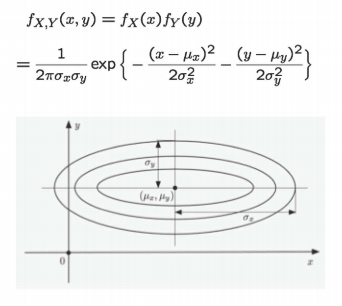
The above figure shows the contours of the joint distribution $f_{X, Y}$. All along the contour, the function has a constant value. Therefore,
\[\begin{align} &\frac{1}{2\pi \sigma_x \sigma_y }\textrm{exp}\bigg\{-\frac{(x-\mu_x)^2}{2\sigma_x^2}-\frac{(y-\mu_y)^2}{2\sigma_y^2}\bigg\} = c &\textrm{for all }x, y \textrm{ on the contour}\\ \implies & -\frac{(x-\mu_x)^2}{2\sigma_x^2}-\frac{(y-\mu_y)^2}{2\sigma_y^2} = k\\ \end{align}\]We know that the equation of an ellipse with center $(x_0, y_0)$ and whose major and minor axes are aligned with the co-ordinate axes, is given as follows:
\[\frac{(x - x_0)^2}{a^2} + \frac{(y - y_0)^2}{b^2} = 1\]Comparing the two equations stated above, we can see that the contours of the joint distribution are elliptical with the center at $(\mu_x, \mu_y)$.
Bayesian Inference is all about infering the value of an unobserved variable $X$ on the basis of an observed variable $Y$. Instead of depending on the prior probability distribution of $X$, given by $p_X(.)$, we depend on the posterior probability distribution $p_{X\mid Y}(.)$ We have seen the Bayes’ Rule for general probability and events. Here we translate it into PMF notation.
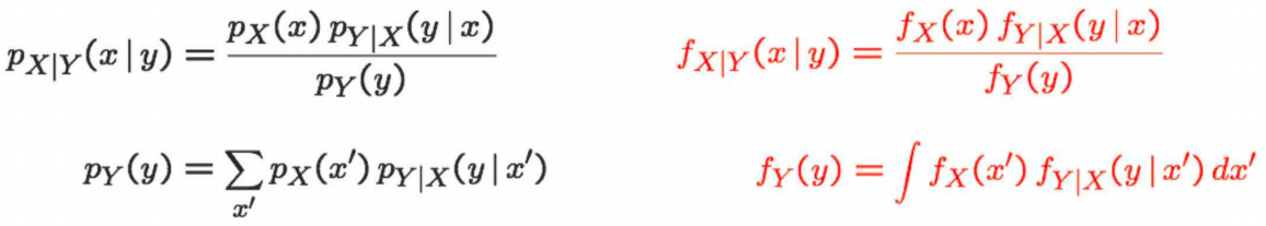
It is not necessary that the observed variable and unobserved variable are both Discrete or Continuous. One might be continuous and the other might be discrete. Bayes’ Rule for these situations can be derived from the definition of Joint Probabilities using similar techniques. See Lec 10.9 for more details.
Finally the lecture covers two scenarios where this Mixed Bayes’ Rule is used. First is the Binary Signal Detection. Here we observe a continuous signal over the wire, and we need to infer whether it is 0 or 1 (discrete). Second is Coin Bias Inference. Here the observed variable is the number of heads (discrete). The variable to be infered (bias) is continuous between 0 and 1.