
Perpetual student. Interested in Maths, Computer Science and Machine Learning.
A probabilistic model is a mathematical description of an uncertain situation. Every probablistic model involves an underlying process, called the experiment, that produces exactly one of several possible outcomes. The set of all possible outcomes is known as the sample space ($\Omega$) of the experiment. A subset of the sample space, that is, a collection of possible outcomes, is called an event.
Probabilistic modeling can usually be broken down into three basic steps:
The probability law must follow the probability axioms of non-negativity, additivity and normalization, stated below:
Non-negativity : $\prob(A)\geq 0, \forall A \subset \Omega$
Additivity : If $A$ and $B$ are disjoint events, then $\prob(A \cup B) = \prob(A) + \prob(B)$
Normalization : The probability of the entire sample space is equal to 1, that is, $\prob(\Omega) = 1$
Based on this the probability of an event $A$ consisting of outcomes $s_1, s_2, \cdots, s_k$, is given as follows:
\[\prob(\{s_1, s_2, s_3, \dots, s_k\}) = \prob(\{s_1\}) + \prob(\{s_2\}) + \prob(\{s_3\}) + \dots + \prob(\{s_k\})\]If the probability of all outcomes (in the entire sample space) is the same then
\[\prob(A)= \frac{(\textrm{no. of elements in }A)}{n}\]Here $A$ is a subset of the sample space and $n$ is the total number of elements in the sample space.
Similar rules apply for continuous models, where instead of talking in terms of particular outcomes, we talk in terms of intervals.
Given an experiment, a corresponding sample space, and a probability law, suppose that we know that the outcome is within some given event $B$. We wish to quantify the likelihood (find the probability) that the outcome also belongs to some other event $A$. We thus seek to construct a new probability law over the updated universe $B$.
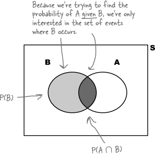
The probability of the outcome belonging to an event $A$, given we already know that event $B$ has occurred, is called the conditional probability of $A$ given $B$, denoted by $\prob(A \mid B)$. From the definition, it is clear that
\[\prob(A \mid B) \propto P(A \cap B)\]The normalizing constant in the above equation, such that $\prob(A \mid B) + \prob(A^c \mid B) = 1$, should be $\prob(A\cap B) + \prob(A^c \cap B) = \prob(B)$. Thus, we have
\[\prob(A \mid B) = \frac{\prob(A \cap B)}{\prob(B)}\]The above equation makes intuitive sense. Out of the total probability assigned to outcomes of event $B$, $\prob(A \mid B)$ gives the fraction of probability that is assigned to outcomes that also belong to event $A$. The equation can be rewritten as:
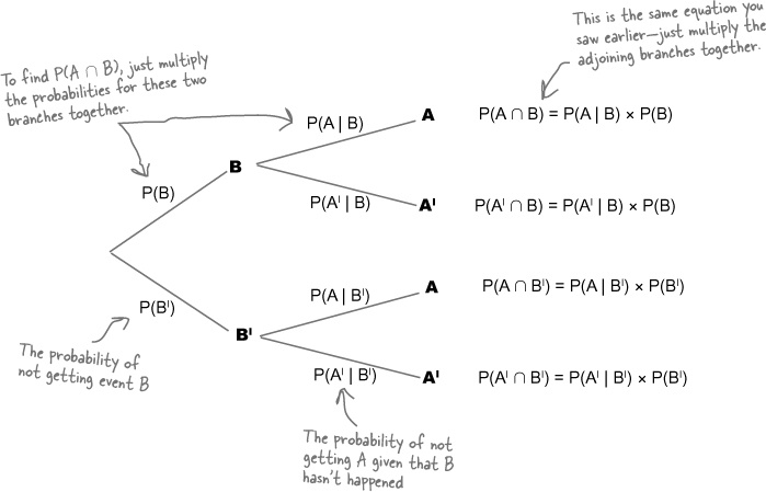
\[\prob(A \cap B) = \prob(B) \times \prob(A \mid B)\]This is called the Product Rule in Probability Theory. How many times $A$ and $B$ occur together? How many times does $B$ occur? Out of the times $B$ occurs, how many times does $A$ occur?
Venn diagrams aren’t always the best way of visualizing conditional probability. A better tool is - a probability tree. Probability trees don’t just help you visualize probabilities; they can help you to calculate them, too. Each branch of the probability tree shows the probability of a particular outcome given the outcome of the parent branch. You can find probabilities involving intersections by multiplying the probabilities of linked branches together. As an example, suppose you want to find $\prob(A \cap B)$. You can find this by multiplying $\prob(B)$ and $\prob(A \mid B)$ together.
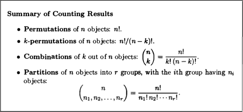
The counting method, which applies to the case where the number of possible outcomes is finite and all outcomes are equally likely. To calculate the probability of an event, we count the number of elements of the event and divide by the number of elements in the sample space. Some useful results, for counting the number of possible outcomes, are as follows:
The sequential method, where we model the problem as a tree. Suitable conditional probabilities are specified along the branches of the probability tree. The probability of various events are then obtained by multiplying conditional probabilities along the corresponding paths of the tree, using the product rule.
The divide and conquer method, where we first calculate $\prob(B \mid A_i)$ i.e. the probability of $B$ happening in different partitions of the sample space, and then combine these probabilities to get the total probability of $B$ happening in the entire sample space.
This is called the Sum Rule in Probability Theory.
Bayes’ Theorem is derived directly from the definition of Conditional Probability. To get a background on Bayesian Inference go through Lec 2.5. Basically we have an event $B$ (which can be recorded/measured, like generation of alarm by a radar). Based on that, we try to infer which condition was true when $B$ happened: $A_1$ (aircraft was present), $A_2$ (goose was present), $A_3$ (the sky was clear) and so on. Therefore we try to calculate $\prob(A_1 \mid B)$, $\prob(A_2\mid B)$, etc.
Bayes’ Theorem says that:
\[\begin{align} \prob(A_i \mid B) &= \frac{\prob(A_i) \prob(B \mid A_i)}{\prob(B)}\\\\ &= \frac{\prob(A_i) \prob(B \mid A_i)}{\sum_j{\prob(A_j)\prob(B \mid A_j)}}\\ \end{align}\]Here,
$\prob(A_i)$, is known as the prior. It is the probability of occurrence of $A_i$, prior to the information that the event $B$ has occurred.
$\prob(B \mid A_i)$ is the likelihood. It is the likelihood of data (observable/recordable event) when $A_i$ event has occurred.
$\prob(A_i \mid B)$ is called the posterior, because by this time the data event has already occurred. We are trying to find the probability of the event $A_i$ having happened back in time; posterior probability.
$\prob(B)$ or $\prob(\text{data})$ doesn’t have a name in general. It is the probability of occurrence of the data event. Generally, data event has some observable/measurable characteristics that helps us calculate its probability of occurrence.
We have introduced the conditional probability $\prob(A \mid B)$ to capture the partial information that event $B$ provides about event $A$. An interesting and important case arises when the occurrence of $B$ provides no such information and does not alter the probability that $A$ has occurred, i.e.,
\[\prob(A \mid B) = \prob(A)\]When we substitute the above equation into the formula for conditional probability $\prob(A \mid B) = \frac{\prob(A \cap B)}{\prob(B)}$, we get
\[\prob(A \cap B) = \prob(A) \times \prob(B)\]Because the above formula is symmetric in $A$ and $B$, we can use it as an alternate definition for independence. Two events are independent if their joint probability (probability of their intersection) is equal to the product of their individual probabilities.
Remember that if two events are independent, they aren’t necessarily conditionally independent and vice-versa. Also, if events $A$, $B$ and $C$ are pairwise independent, it doesn’t mean that they are actually independent i.e. $\prob(A \cap B \cap C)$ is not necessarily equal to $\prob(A) \times \prob(B) \times \prob(C)$, if $A$, $B$ and $C$ are pairwise independent.