
Perpetual student. Interested in Maths, Computer Science and Machine Learning.
We are now equipped with the basics of Linear Algebra. We are familiar with how a matrix can be used to represent a vector space, as well as a system of linear equations. Now let us try to apply this knowledge to learn from data (aka Machine Learning). We will be relying on ECE 532 and MIT 18.06 for the same.
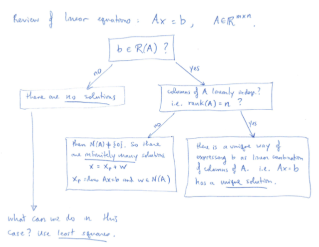
Machine Learning Setup : We’d like to solve $A \bt{x} = \bt{b}$, where:
Typically $A$ will be full rank and $\bt{b} \notin \bt{R}(A)$; so there is no solution that would satisfy all the equations. We define the residual $\bt{r} = A\bt{x} - \bt{b}$.
Because we can’t make $\bt{r} = \bt{0}$ ($A\bt{x} = \bt{b}$ has no solutions), instead we try to make \(\|\bt{r}\|\) as small as possible, often written as
\[\min_\bt{x}{\|A\bt{x} - \bt{b}\|^2}\]Geometrically, we want to find a vector in the column space of $A$ (represented by $A\bt{x}$) which has the least square distance from $\bt{b}$. Let \(\hat{\bt{x}} = \textrm{argmin}_\bt{x}{\|A\bt{x} - \bt{b}\|^2}\). By Pythagoras Theorem, the minimum residual $\hat{\bt{r}}$ will be perpendicular to $\bt{R}(A)$ ( perpendicular to all the vectors in $\bt{R}(A)$).
Thus, in order to deal with least squares, we need to have background in orthogonality and projections. And that is exactly what we will develop next.
What does it mean for two subspaces / vectors / basis to be orthogonal?
Vector Orthogonality: Two vectors $\bt{x}$ and $\bt{y}$ are orthogonal iff $\bt{x}\cdot\bt{y} = 0$ or in other words, $\bt{x}^T\bt{y}=0$.
Subspace orthogonality: Two subspace $\bt{S}$ and $\bt{T}$ are orthogonal to each other, when every vector in $\bt{S}$ is orthogonal to every vector in $\bt{T}$.
Are two perpendicular planes in $\mathbb{R}^3$ orthogonal to each other? No. Vectors in the intersection set are not orthogonal. Two orthogonal subspaces will have only $\bt{0}$ in their intersection set.
Null space & Row space of a $m \times n$ matrix are both spaces in $\mathbb{R}^n$ and are orthogonal to each other. Why?
\[\bt{x} \in \bt{N}(A) \iff A\bt{x} = \mat{\bt{r_1} \cdotp \bt{x}\\ \vdots \\\bt{r_n} \cdotp \bt{x}} = \mat{0 \\ \vdots \\ 0}\]We mentioned that the minimum residual $\hat{\bt{r}}$ will be perpendicular to the column space of $A$. This can be written as $\hat{\bt{r}} \in \bt{R}(A)^\perp$. The set $S^\perp$ ($S$ perp) is defined as the set of all vectors that are perpendicular to $S$.
\[S^\perp = \{ \bt{w} \in \mathbb{R}^n | \bt{w}^T\bt{x} = \bt{0},\; \forall \bt{x} \in S\}\]This set defines a vector space, because:
This leads to following definition:
Orthogonal Complement: If a subspace $\bt{V}$ contains all the orthogonal vectors to another subspace $\bt{T}$, then $\bt{V}$ is called orthogonal complement of $\bt{T}$, denoted by $\bt{T}^\perp$ ($\bt{T}$ perp).
Null space & Row space of a matrix are not only orthogonal, but are also orthogonal complements of each other. Nullspace contains all vectors orthogonal to the row space.
Let us start by considering the projection of a vector $\bt{b}$ on another vector $\bt{a}$. Let $\bt{p}$ be the projected vector. This projection vector will be in the direction of $\bt{a}$, so $\bt{p} = k\bt{a}$.
Then,
\[\begin{align} &(\bt{b} - \bt{p}) \perp \bt{a} \\ \implies &\bt{a}^T(\bt{b} - \bt{p}) = 0 \\ \implies &\bt{a}^T(\bt{b} - k\bt{a}) = 0 \\ \implies &\bt{a}^T\bt{b} - k\bt{a}^T\bt{a} = 0\\ \implies &\bt{a}^T\bt{a}k = \bt{a}^T\bt{b} &\textrm{normal equation in 1D, } k\leftrightarrow \hat{\bt{x}}\\ \implies &k = \frac{\bt{a}^T\bt{b}}{\bt{a}^T\bt{a}} & \bt{a}^T\bt{a}\textrm{ is a scalar} \\ \implies &\bt{p} = k\bt{a} = \bt{a}k = \bt{a}\frac{\bt{a}^T\bt{b}}{\bt{a}^T\bt{a}} = \frac{\bt{a}\bt{a}^T}{\bt{a}^T\bt{a}}\bt{b} = P\bt{b}\\ \end{align}\]The matrix $\frac{\bt{a}\bt{a}^T}{\bt{a}^T\bt{a}}$ is called the Projection Matrix $P$. Note that $\bt{a}\bt{a}^T$ is a $3 \times 3$ matrix, not a number; matrix multiplication is not commutative.
Now let us come to our original problem statement of finding an $\hat{\bt{x}}$ such that the norm of $\hat{\bt{r}} = A\hat{\bt{x}} - \bt{b}$ is minimized. $\hat{\bt{r}} \in \bt{R}(A)^\perp$, so it orthogonal to each column vector of $A$. Therefore
\[\begin{align} & A^T\hat{\bt{r}} = 0\\ \implies & A^T(A\hat{\bt{x}} - \bt{b}) = 0 \\ \implies & A^TA\hat{\bt{x}} = A^T\bt{b} &\textrm{Normal Equations}\\ \end{align}\]$A^TA$ is a $n\times n$ matrix ($n$ is the number of independent variables). The normal equations give a system of $n$ linear equations with $n$ unknowns.
Fact: $A^TA$ is invertible (i.e. $A^TA\hat{\bt{x}} = A^T\bt{b}$ has a unique solution) if and only if $A$ has linearly independent columns (i.e. rank($A$) = n, or $\bt{N}(A) = \bt{0}$).
Proof: Observe that if $A\bt{x} = \bt{0}$ for some $\bt{x}$, then $A^TA\bt{x} = \bt{0}$. Similarly if $A^TA\bt{x} = \bt{0}$, then $\bt{x}^T A^TA\bt{x} = \bt{0}$ and \(\|A\bt{x}\| = 0\), which implies $A\bt{x} = \bt{0}$.
\[\bt{N}(A) = \bt{N}(A^TA) \\ \therefore \bt{N}(A) = \{\bt{0}\}\iff \bt{N}(A^TA) = \{\bt{0}\}\]Conclusion: If $A$ has linearly independent columns, then solution to least square problem \(\min \|A\bt{x} - \bt{b}\|^2\) is
\[\hat{\bt{x}} = (A^TA)^{-1}A^T\bt{b}\]The projection is given by
\[A\hat{\bt{x}} = A(A^TA)^{-1}A^T\bt{b}\]$A(A^TA)^{-1}A^T$ is called the projection matrix $P$ of $A$.
Important Fact: If $P$ is the projection matrix of $A$, then $P^2\bt{x} = P\bt{x}$ and $P^2 = P$. Why? Because $P\bt{x} \in \bt{R}(A)$ and $\textrm{proj}_{\bt{R}(A)}P\bt{x} = P\bt{x}$.
If $A$ is not invertible then $\hat{\bt{x}} = \hat{\bt{x}}_1 + \bt{w}$, where $\hat{\bt{x}}_1$ is a solution to the normal equations and $\bt{w} \in \bt{N}(A)$.
Aside: If $A$ is an invertible square matrix, then $P$ becomes $I$ (identity matrix). This is because $\bt{b}$ will always be in the column space of $A$ if $A$ is an invertible square matrix.
Suppose we have three data-points $(x_i, y_i) = (1,1),(2,2),(3,2)$ and we want to fit a linear model ($y_i = mx_i + c$) to our data.
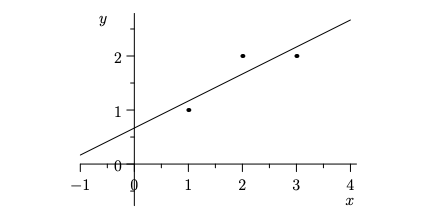
Our system of linear equations is given by:
\[\begin{align} \mat{1 & 1 \\ 2 & 1 \\ 3 & 1} \mat{m \\ c} &= \mat{1 \\2 \\ 2} \\ A \bt{x} &= \bt{b} \end{align}\]Here $A$ is a long matrix. So for many $\bt{b}$(s) there won’t exist any solution (there won’t be a single line passing through all the points). Therefore we find the projection of $\bt{b}$ on $\bt{R}(A)$. That projection will be the closest point to $\bt{b}$ that can be achieved by a linear model.
If the columns of $A$ are independent (two features are not linearly correlated) then we have a unique solution for \(\bt{x} = \mat{m \\ c}\) which is given by $\hat{\bt{x}} = (A^TA)^{-1}A^T\bt{b}$. If a column of $A$ is a linearly scaled version of another column, then there can be multiple solutions (this is the case when we perform Regression with highly correlated variables).
Once we have found a solution \(\hat{\bt{x}} = \mat{\hat{m}\\ \hat{c}}\), for any new point you can use the linear model to make predictions. Just plug the value of $x_{new}$ in the model ($y_{new} = \hat{m}x_{new} + \hat{c}$).
Additional Links
For a more real life version of Linear Regression refer to Lecture 5 (pg-8) of ECE-532.
For a matrix calculus oriented way of deriving $\hat{\bt{x}}$ refer to Lecture 6 (notes) of ECE-532. Don’t go through the second half of the lecture.
The same technique of least squares can also be used to build a model for Linear Classification. For details refer to Lecture 8 (notes) of ECE-532.
A set of orthonormal vectors \(\{\bt{q_1}, \bt{q_2},\dots\}\) is a set of unit vectors where every pair is perpendicular. We can represent this as a matrix $Q = \mat{\bt{q_1} & \bt{q_2} & \dots}$, where $\bt{q_i}$(s) are column vectors. The above requirement can be written as $Q^TQ=I$. This matrix $Q$ is called an orthonormal matrix.
Property 1: If $Q$ is an orthonormal matrix, then $|Q\bt{x}| = |\bt{x}|$.
Proof: $|Q\bt{x}|^2 = (Q\bt{x})^T(Q\bt{x}) = \bt{x}^TQ^TQ\bt{x} = \bt{x}^T\bt{x} = |\bt{x}|^2$
Also,
\[\begin{align} (Q\bt{x})^T (Q\bt{y}) &= (\bt{x}^T Q^T) (Q \bt{y}) \\ &= \bt{x}^T (Q^T Q) \bt{y} \\ &= \bt{x}^T \bt{y} \end{align}\]The magnitude of each vector, and angle between each pair of vectors is maintained. Thus, multiplication by $Q$ just rotates the entire vector space.
Property 2: If $Q$ is orthonormal, then the Projection Matrix
\[\begin{align} P &= Q(Q^TQ)^{-1}Q^T \\ &= Q(I)^{-1}Q^T \\ &= QQ^T \\ \end{align}\]Remember that $QQ^T$ is not equal to the Identity Matrix, when $Q$ is non-square.
What happens when $Q$ is square? We have $ Q^TQ=I = QQ^T$ and $Q^{-1} = Q^T$.
How do we find the orthonormal basis for $\bt{R}(A)$? Gram-Schmidt Algorithm does that for you.

Psuedocode:
Normalize $\bt{a_1}$, and include it in the result set $U$.
$\forall \bt{a_i}\in A$ {
$\quad\quad\forall \bt{u}\in U$ {
$\quad\quad\quad\quad\bt{a_i} = \bt{a_i} - (\bt{u}^T\bt{a_i}){\bt{u}} \quad\quad $ (remove the projection of $\bt{a_i}$ on $\bt{u}$)
$\quad\quad$}
$\quad\quad$ if $(\bt{a_i} \neq \bt{0}$): $U = U \cup {\frac{\bt{a_i}}{|\bt{a_i}|}}$
}
Notice that any vector $\bt{a_k}$ that lives in the span of ${\bt{a_1}, \bt{a_2}, \dots, \bt{a_{k-1}}}$ will automatically be converted to $\bt{0}$ and will be excluded from $U$.
If $\bt{S} \subset \mathbb{R}^n$ is any subspace, we can find orthonormal $U_1 \in \mathbb{R}^{n \times r}$ such that $\bt{R}(U_1) = \bt{S}$ using Gram Schmidt. We can also find $U_2$ such that $U = \mat{U_1 & U_2}$ is orthonormal and $U$ spans the entire $\mathbb{R}^n$ ($U$ is square). How? Apply Gram Schmidt on $\mat{U_1 & I}$. The extra rows will drop, as explained above.
But why is finding an Orthonormal Basis so important? The reason is as follows:
Suppose we want to find the projection of $\bt{b}$ on $\bt{R}(A)$. Suppose $Q$ is an orthonormal matrix such that $\bt{R}(A) = \bt{R}(Q)$. Then, \(\textrm{proj}_{\bt{R}(A)}\bt{b} = \textrm{proj}_{\bt{R}(Q)}\bt{b}\).
\[\begin{align} \textrm{proj}_{\bt{R}(Q)}\bt{b} &= (QQ^T)\bt{b} \\ &= Q(Q^T\bt{b}) \\ &= \bt{q_1}\bt{q_1}^T\bt{b} + \bt{q_2}\bt{q_2}^T\bt{b} + \dots + \bt{q_r}\bt{q_r}^T\bt{b} \\ &= \textrm{proj}_{\bt{q_1}}\bt{b} + \textrm{proj}_{\bt{q_2}}\bt{b} + \dots + \textrm{proj}_{\bt{q_r}}\bt{b} \\ \end{align}\]Thus, if $Q$ is an orthonormal basis, then calculating projection of $\bt{b}$ on $\bt{R}(Q)$ is the same as combining the projections of $\bt{b}$ on each of the basis vectors individually. This equation is very easy to compute (it is just the dot product of two vectors, $\bt{b}$ and $\bt{q_i}$). With orthonormal basis, calculating projections becomes almost trivial.